The Hidden Problem: Missing Data leads to biased SBI posteriors
Simulation-based inference (SBI) has proven remarkably successful for fitting complex models when likelihoods are intractable [Cra20F]. From gravitational wave astronomy to computational neuroscience, SBI methods enable parameter inference for models where simulation is feasible but likelihood computation is not. However, most SBI methods assume complete observations, while real-world data often contains missing values due to instrument limitations, recording failures, or experimental constraints.
As [Ver25R] demonstrate in Figure 1, naive approaches to handling missing data lead to increasingly biased posteriors as the proportion of missing values grows. Even with just 10% missing values, posterior estimates begin drifting from true parameters. At 60% missingness, the bias becomes severe, potentially invalidating scientific conclusions.
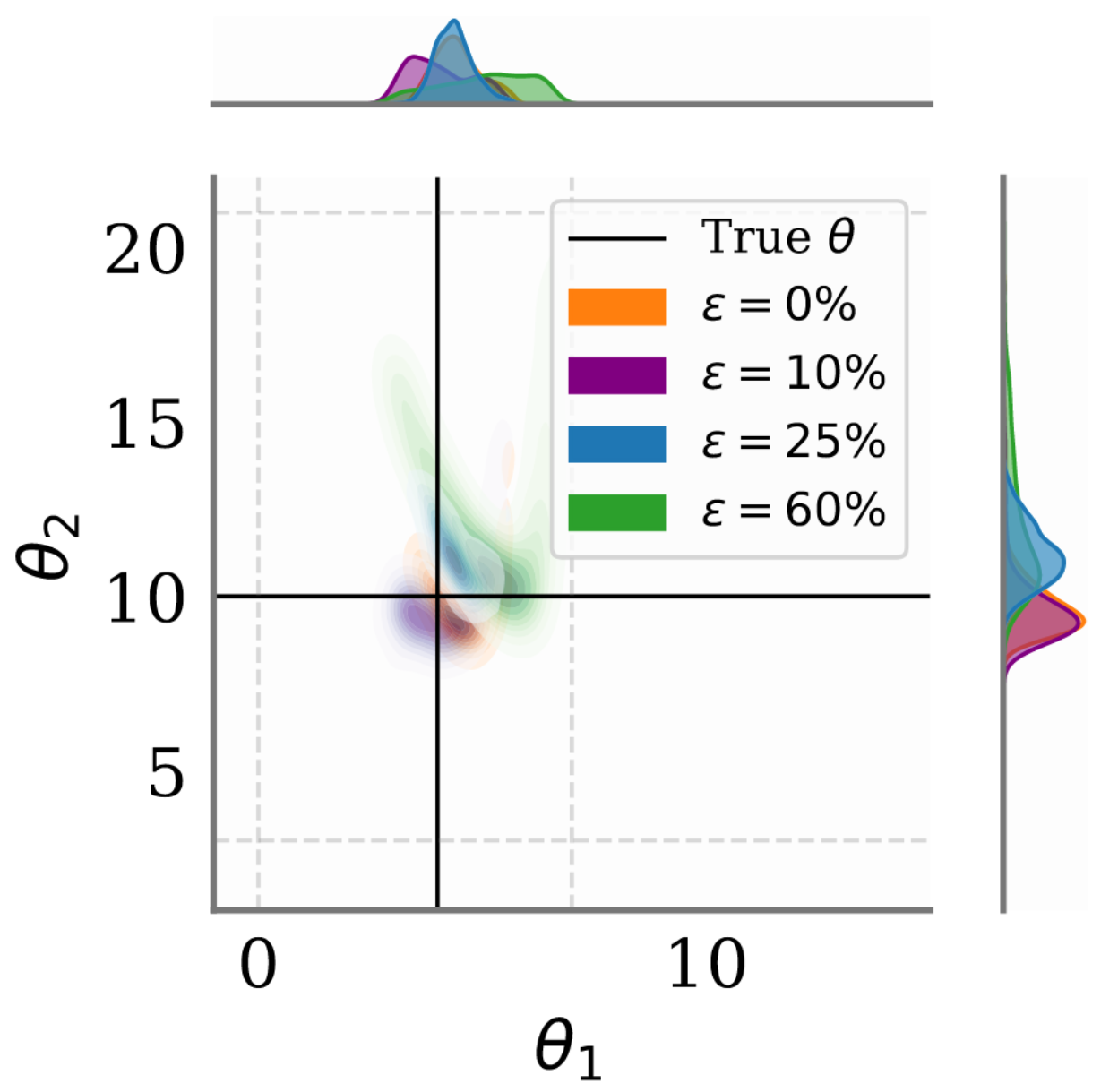 Figure 1 [Ver25R]: Effect of missing data on
neural posterior estimation. As the proportion of missing values ε increases, SBI
posteriors learned with naive missing data handling (here zero imputation) become
increasingly biased and drift away from the true parameter value (solid lines). This
example uses the Ricker population model.
Figure 1 [Ver25R]: Effect of missing data on
neural posterior estimation. As the proportion of missing values ε increases, SBI
posteriors learned with naive missing data handling (here zero imputation) become
increasingly biased and drift away from the true parameter value (solid lines). This
example uses the Ricker population model.While the landscapte of SBI methods has advanced significantly over the last couple of years, systematic treatment of missing data has received limited attention until recently.
Understanding the Types of Missingness
Not all missing data is created equal. The statistical properties of missing data depend fundamentally on the mechanism that causes values to be missing. [Rub75I] formalized this insight by categorizing missingness into three distinct types, each with different implications for inference:
- MCAR (Missing Completely at Random): The probability of missingness is independent of both observed and unobserved data. Example: sensor failures due to random power outages.
- MAR (Missing at Random): Missingness depends only on the observed data. Example: older patients being more likely to miss follow-up appointments, where age is observed.
- MNAR (Missing Not at Random): Missingness depends on the unobserved value itself – the most challenging scenario. Example: high blood pressure readings causing device malfunctions.
Methods that do not account for the underlying missingness mechanism are prone to bias, particularly in MAR and MNAR cases. In the context of SBI, this means that the imputation strategy (replacing missing values with predicted values) must be tailored to the type of missingness to avoid systematically distorting the posterior.
Why is missing data problematic for neural SBI methods?
One of the predominant SBI techniques is neural posterior estimation (NPE, [Pap18F]). NPE approximates the posterior using conditional density estimation: A neural density estimators $q_\psi(\theta|x)$, e.g., a normalizing flow parametrized by $\psi$, learns to approximate the unknown posterior $p(\theta | x)$ using simulated data. When at inference time with real data we naively impute missing values, we create data patterns that the network has never encountered during training – effectively out-of-distribution inputs. Neural networks are notoriously unreliable when presented with such inputs, potentially producing arbitrarily incorrect posterior estimates. This is more severe than in classical statistical methods because neural networks do not just interpolate poorly; they can fail catastrophically.
Several attempts have been made to address missing data in SBI contexts. [Lue17F] extended the standard NPE approach by learning an imputation model at the last layer of the inference network, though without explicitly modeling the missingness mechanism. [Wan24M] explored augmenting missing values with constants (zeros or sample means) and including binary masks as additional inputs to NPE. While computationally simple, this approach can introduce systematic biases and fails to capture imputation uncertainty.
More recently, [Glo24A] introduced the Simformer, a transformer-based architecture that can perform arbitrary conditioning on partially observed data. While powerful, this method requires substantial computational resources and does not explicitly model different missingness mechanisms (MCAR, MAR, MNAR).
These approaches highlight a fundamental challenge: imputation and inference are interdependent problems. Accurate imputation requires understanding the data distribution, which in SBI depends on the parameters being inferred. Conversely, accurate inference requires complete data or principled handling of missingness.
RISE: Joint Learning of Imputation and Inference
The key insight of RISE (Robust Inference under imputed SimulatEd data) is that imputation and inference should be learned jointly within a unified framework. Rather than treating these as sequential steps, RISE simultaneously learns a distribution over missing values and a parameter posterior that marginalizes over imputation uncertainty.
Theoretical Foundation
Given observed data $x_{\text{obs}}$ and missing data $x_{\text{mis}}$, the posterior over simulator parameters $\theta$ given observed data can be expressed as:
$$p(\theta | x_{\text{obs}}) = \int p(\theta | x_{\text{obs}}, x_{\text{mis}}) p(x_{\text{mis}} | x_{\text{obs}}) dx_{\text{mis}}$$
The integral is composed of two important components: the posterior given complete data $p(\theta | x_{\text{obs}}, x_{\text{mis}})$ (what standard NPE approximates) and the imputation distribution $p(x_{\text{mis}} | x_{\text{obs}})$. [Ver25R] show that using an incorrect imputation distribution $\hat{p}(x_{\text{mis}} | x_{\text{obs}})$ leads to biased posteriors, with bias proportional to the divergence between true and estimated imputation distributions.
The RISE Framework
To learn the posterior and the imputation model jointly, RISE extends the common NPE loss function with an additional term that optimizes the missing model. The standard NPE loss is given by
$$\min_{\phi,\psi} -\mathbb{E}_{\theta, x \sim p(x|\theta)p(\theta)} \log q_\psi(\theta|x),$$
which encourages the network to assign high probability to the parameters $\theta$ that generated the corresponding (simulated) data $x$. The joint RISE loss, taking into account missing and observed data, is then defined as:
$$\min_{\phi,\psi} -\mathbb{E}_{(x_{\text{obs}}, \theta)} \mathbb{E}_{x_{\text{mis}} \sim p(x_{\text{mis}}|x_{\text{obs}})} \left[\log \hat{p}_\phi(x_{\text{mis}}|x_{\text{obs}}) + \log q_\psi(\theta|x_{\text{obs}}, x_{\text{mis}})\right].$$
Here, $\hat{p}_\phi$ learns to predict missing values given observations, while $q_\psi$ estimates the parameter posterior. The joint training ensures that each network learns in the context of the other, capturing the interdependencies between imputation and inference.
Neural Processes for Flexible Imputation
RISE employs Neural Processes (NP) [Gar18C] as its imputation model (\hat p_\phi), which allows it to learn distributions over functions rather than point predictions. This makes NPs well suited for imputing missing data, as they naturally capture uncertainty and correlations between observed and missing entries.
Intuition: Consider a time series where some voltage measurements are missing. Each observed value $x_{\text{obs}}$ is paired with a location index $c_{\text{obs}}$ (e.g., its time point). These pairs form a context set $C = {(c_{\text{obs}}, x_{\text{obs}})}$. The NP encoder summarizes this context into a latent distribution, and the decoder then predicts a distribution for the missing values $x_{\text{mis}}$ at their indices $c_{\text{mis}}$. In this way, the imputer treats the data as a function from index to value and learns how to interpolate or extrapolate missing entries with calibrated uncertainty.
The predictive distribution is:
$$\hat{p}_\phi(x_{\text{mis}} | c_{\text{mis}}, C) = \int \hat{p}_\alpha(x_{\text{mis}} | c_{\text{mis}}, \tilde{z}) \hat{p}_\beta(\tilde{z} | C) d\tilde{z}$$
where the latent variable $\tilde z$ captures structure in the observed data and, crucially, the missingness pattern. To support different missingness mechanisms, RISE factorizes $\tilde z = (z, s)$, where $z$ encodes correlations in the data and $s$ encodes which entries are missing:
- MCAR: $\hat{p}_\beta(\tilde{z} | x_{\text{obs}}) = p_{\beta_1}(z | x_{\text{obs}})p_{\beta_2}(s)$ - the missingness mask distribution $p_{\beta_2}(s)$ is independent of any data.
- MAR: $\hat{p}_\beta(\tilde{z} | x_{\text{obs}}) = p_{\beta_1}(z | x_{\text{obs}})p_{\beta_2}(s | x_{\text{obs}})$ - the mask depends only on observed values.
- MNAR: $\hat{p}_\beta(\tilde{z} | x_{\text{obs}}) = p_{\beta_1}(z | x_{\text{obs}}) \int p_{\beta_2}(s | x_{\text{mis}}, x_{\text{obs}})p(x_{\text{mis}} | x_{\text{obs}})dx_{\text{mis}}$ - requires marginalizing over the circular dependency between missing values and their missingness.
During training, you choose the missingness assumption (MCAR, MAR, or MNAR), and RISE simulates complete data, constructs missing data by applying masks accordingly, and trains $\hat p_\phi$ on the resulting $(x_{\text{obs}}, x_{\text{mis}})$ pairs. The NP latent structure enables the model to learn the dependencies implied by the chosen mechanism, including MNAR-style dependence on unobserved values. At inference, no mechanism parameters need to be provided—the trained model handles imputation directly from observed data.
Empirical Results and Validation
RISE was evaluated across multiple standard SBI benchmark tasks as well as several real-world datasets.
On standard SBI benchmarks [Lue21B], RISE consistently achieves superior performance metrics compared to baselines including NPE-NN (NPE with feed-forward neural network imputation), the mask-based method of [Wan24M], and the Simformer [Glo24A]. We highlight the most significant improvements for each benchmark.
As common in the SBI literature, performance is measured as C2ST (Classifier Two-Sample Test) score, measuring how distinguishable the estimated posterior is from the true posterior (0.5 is ideal, 1.0 worst), NLPP (Negative Log Posterior Probability) measuring the log probability of true parameters under the estimated posterior (higher is better), and MMD (Maximum Mean Discrepancy), quantifying the distance between distributions (lower is better).
- Gaussian Linear Uniform (GLU): With 60% MCAR missingness, baseline methods achieve C2ST scores of 0.97-0.98 (far from the ideal 0.5), while RISE reaches 0.93-a notably small improvement that indicates slightly better posterior approximation in severe missingness scenarios.
- Generalized Linear Model (GLM): RISE improves NLPP from -8.97 (baseline) to -8.71 under 60% MCAR.
- Two Moons: MMD reduced by 30-40% compared to mask-based approaches across all missingness levels.
The improvements are more pronounced under MNAR conditions, where baseline methods fail to account for the missingness mechanism (see Table 1 in main paper for detailed results).
Figure 2 illustrates performance on the Hodgkin-Huxley model, a complex neuroscience simulator with 1200-dimensional voltage trace observations. While baseline methods (NPE-NN) show increasing bias with more missing data, RISE maintains accurate posteriors even at 60% missingness.
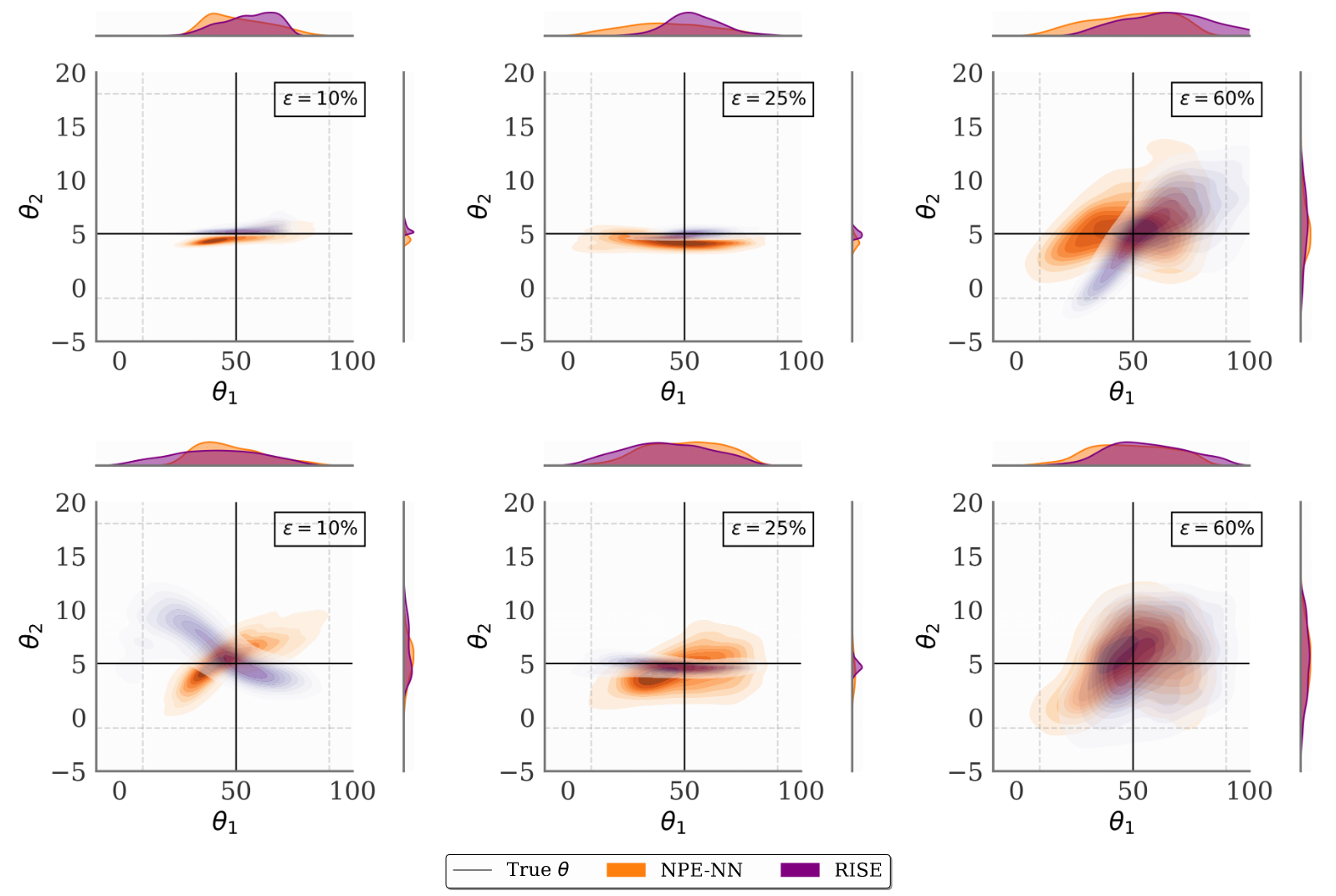
Figure 2 [Ver25R]: Posterior estimates for the Hodgkin-Huxley neuron model under MCAR (top) and MNAR (bottom) missingness, shown for the baseline NPE (blue) and the proposed method RISE (green).
Computational Considerations
Despite jointly training two networks, RISE adds only modest computational overhead of approximately 50% more training time than standard NPE. Once trained, the method remains fully amortized: new observations with missing data require only forward passes through both networks. Memory requirements scale linearly with the proportion of missing values, making the approach practical for moderate-dimensional problems.
Limitations and Extensions
The empirical evaluations show only marginal improvements compared to baseline methods when compared in terms of C2ST posterior accuracy. When compared via MMD or NLPP, the improvemets were more pronounced, which could be explained by higher sensitivity of C2ST in some posterior dimensions. This should be investigated in follow-up studies.
RISE inherits potential calibration issues from NPE [Her23C], which may be compounded by imputation uncertainty. The Neural Process component assumes Gaussian predictive distributions, potentially limiting flexibility for highly non-Gaussian data. Current implementation treats all missing values equally, though some measurements may be more informative than others.
Scope and Applicability
RISE makes several key assumptions that define when it can be effectively applied:
Well-specified simulator: The method assumes the simulator accurately represents the true data-generating process. Extensions to handle model misspecification remain future work.
Missingness mechanism assumption: During training setup, you choose which missingness assumption (MCAR, MAR, or MNAR) governs the simulated training masks based on domain knowledge. Given this assumption, RISE automatically learns the mechanism parameters and conditional dependencies through its latent Neural Process. At inference, the learned mechanism is handled implicitly—no manual specification needed. However, RISE cannot automatically determine which of the three assumptions best fits your real-world problem; that choice must be informed by domain expertise.
Moderate missingness levels: Empirical validation covers up to 60% missing data. Performance under extreme missingness (>70%) remains uncharacterized.
Moderate-dimensional data: Memory requirements scale linearly with missing value proportion, making the approach most practical for problems with moderate dimensionality.
For practitioners: RISE is most suitable when you have (1) a trusted simulator, (2) domain knowledge to select the appropriate missingness assumption for training, and (3) missingness levels up to ~60% in moderate-dimensional settings. Once trained under your chosen assumption, RISE handles the mechanism automatically at inference time.
Future extensions could address these limitations through several avenues. Alternative imputation architectures (e.g., normalizing flows or diffusion models) might provide more flexible distributions. Importance-weighted schemes could prioritize critical measurements. Extension to other SBI algorithms beyond NPE would broaden applicability.
The method is implemented in PyTorch and available at https://github.com/Aalto-QuML/RISE.
