The dynamic behavior of physical systems is often described by conservation and constitutive laws, expressed as systems of partial differential equations (PDEs). A classical task involves the use of computational tools to solve such equations across a range of scenarios, e.g., different domain geometries, input parameters, and initial and boundary conditions. Solving these so-called parametric PDEs using traditional tools (e.g., finite element methods) comes with an enormous computational cost, as independent simulations need to be performed for every different domain geometries or input parameter.
In the noteworthy paper [Wan21L], the authors propose the framework of physics-informed DeepONets for solving parameterized PDEs. It is a simple yet remarkably effective extension of the DeepONet framework [Lu21L] (cf. Learning nonlinear operators: the DeepONet architecture). By constraining the outputs of a DeepONet to approximately satisfy an underlying governing law, substantial improvements in predictive accuracy, enhanced generalization performance even for out-of-distribution prediction, as well as enhanced data efficiency can be observed.
 Figure 1 [Wan21L]: Making DeepONets physics
informed. The DeepONet architecture consists of two subnetworks, the branch net
for extracting latent representations of input functions and the trunk net for
extracting latent representations of input coordinates at which the output
functions are evaluated. A continuous and differentiable representation of the
output functions is then obtained by merging the latent representations
extracted by each subnetwork via a dot product. Automatic differentiation can
then be used to formulate appropriate regularization mechanisms for biasing the
DeepONet outputs to satisfy a given system of PDEs. BC, boundary conditions; IC,
initial conditions.
Operator learning techniques have demonstrated early promise across a range of
applications, but their application to solving parametric PDEs faces two
fundamental challenges: First, they require a large corpus of paired
input-output observations and, second, their predicted output functions are not
guaranteed to satisfy the underlying PDE. Motivated by the fact that the outputs
of a DeepONet model are differentiable with respect to their input coordinates,
one can use automatic differentiation to formulate an appropriate regularization
mechanism in the spirit of physics-informed neural networks [Rai19P]. The target output functions of the DeepONet
are biased to satisfy the underlying PDE constraints by incorporating these into
the loss function of the network.
Figure 1 [Wan21L]: Making DeepONets physics
informed. The DeepONet architecture consists of two subnetworks, the branch net
for extracting latent representations of input functions and the trunk net for
extracting latent representations of input coordinates at which the output
functions are evaluated. A continuous and differentiable representation of the
output functions is then obtained by merging the latent representations
extracted by each subnetwork via a dot product. Automatic differentiation can
then be used to formulate appropriate regularization mechanisms for biasing the
DeepONet outputs to satisfy a given system of PDEs. BC, boundary conditions; IC,
initial conditions.
Operator learning techniques have demonstrated early promise across a range of
applications, but their application to solving parametric PDEs faces two
fundamental challenges: First, they require a large corpus of paired
input-output observations and, second, their predicted output functions are not
guaranteed to satisfy the underlying PDE. Motivated by the fact that the outputs
of a DeepONet model are differentiable with respect to their input coordinates,
one can use automatic differentiation to formulate an appropriate regularization
mechanism in the spirit of physics-informed neural networks [Rai19P]. The target output functions of the DeepONet
are biased to satisfy the underlying PDE constraints by incorporating these into
the loss function of the network.
When the collection of all trainable weights of a DeepONet is denoted by $\theta$, the network is optimized with respect to the loss function $$ \mathcal{L}(\theta) = \mathcal{L}{\small\text{operator}}(\theta) + \mathcal{L}{\small\text{physics}}(\theta) $$ where $\mathcal{L}{\small\text{operator}}$ fits the available solution measurements and $\mathcal{L}{\small\text{physics}}$ enforces the underlying PDE constraints.
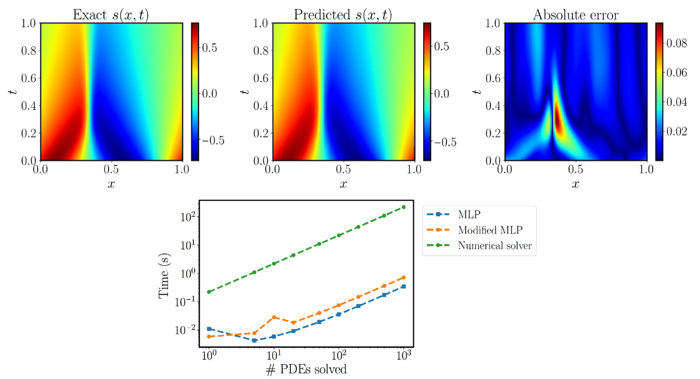
Figure 4 [Wan21L]: Solving a parametric Burgers’ equation. (Top) Exact solution versus the prediction of the best-trained physics-informed DeepONet. The resulting relative L2 error of the predicted solution is 3%. (Bottom) Computational cost (s) for performing inference with a trained physics-informed DeepONet model [conventional or modified multilayer perceptron (MLP) architecture], as well as corresponding timing for solving a PDE with a conventional spectral solver (58). Notably, a trained physics-informed DeepONet model can predict the solution of $O(10^3)$ time-dependent PDEs in a fraction of a second, up to three orders of magnitude faster compared to a conventional PDE solver. Reported timings are obtained on a single NVIDIA V100 graphics processing unit (GPU).
The authors demonstrate the effectiveness of the physics-informed DeepONets in solving parametric ordinary differential equations, diffusion-reaction and Burgers’ transport dynamics, as well as advection and Eikonal equations. In the diffusion-reaction example, the physics-informed DeepONet yields ∼80% improvement in prediction accuracy with 100% reduction in the dataset size required for training. For Burgers’ equation, notably, a trained physics-informed DeepONet model can predict the solution up to three orders of magnitude (1000x) faster compared to a conventional solver.
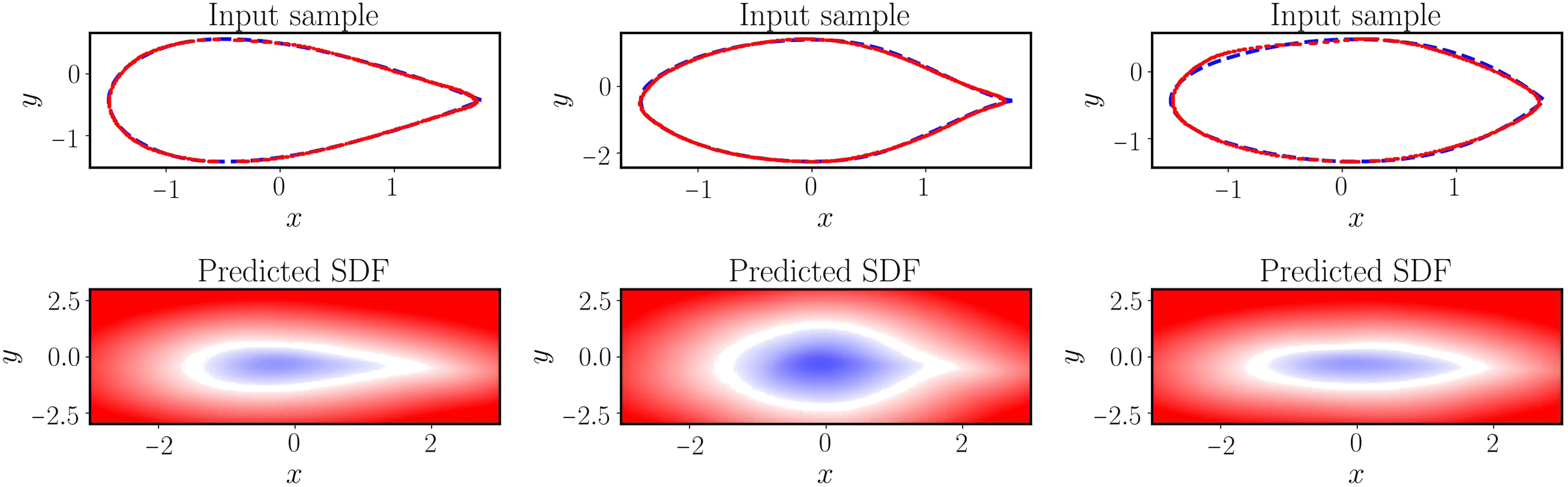
Figure 6 [Wan21L]: Solving a parametric eikonal equation (airfoils). (Top) Exact airfoil geometry versus the zero-level set obtained from the predicted signed distance function for three different input examples in the test dataset. (Bottom) Predicted signed distance function of a trained physics-informed DeepONet for three different airfoil geometries in the test dataset.
Despite the promise of the framework demonstrated in the paper, the authors acknowledge that many technical questions remain. For instance, for a given parametric governing law: What is the optimal feature embedding or network architecture of a physics-informed DeepONet? Addressing these questions might not only enhance the performance of physics-informed DeepONets, but also introduce a paradigm shift in how we model and simulate complex physical systems.
If you are interested in using physics-informed DeepONets (and other physics-informed neural operators) in your application, check out continuiti, our Python package for learning function operators with neural networks that includes utilities for implementing PDEs in the loss function.
