Introduction
Simulation-based inference (SBI) provides a powerful framework for applying Bayesian inference to study complex systems where direct likelihood computation is infeasible [Cra20F]. By using simulated data to approximate posterior distributions, SBI has found applications across diverse scientific fields, including neuroscience, physics, climate science and epidemiology [Gon20T, Bre20S, Wat21M, Wit20S]. However, these methods often assume that the simulator is a faithful representation of the true data-generating process. In practice, this assumption is frequently violated, leading to model misspecification. In this blog post, we provide an overview of the currently available approaches to detect and mitigate model misspecification in SBI, and discuss open challenges.
In standard Bayesian inference, model misspecification can lead to biased or misleading posterior estimates. However, in neural SBI, the problem is particularly severe because the posterior or likelihood is approximated using neural networks trained on simulated data. Neural networks are known to produce arbitrarily incorrect predictions when probed with out-of-distribution (OOD) data [Sze14I], and in a misspecified simulator, the observed data $\mathbf{x}_o$ is effectively OOD relative to the training distribution. This can lead to highly unreliable posterior estimates, distorted uncertainty quantification, and incorrect scientific conclusions.
An illustrative example of model misspecification has been provided by Ward et al. (2022) [War22R] using a simplified version of the Susceptible, Infected, Recovered (SIR) modelt that is commonly used in epidemiology. This simulator estimates key parameters such as the infection rate $\beta$ and recovery rate $\gamma$, with observations summarized by metrics like the maximum number of infections, timing of peak infection, and autocorrelation. In this setting, misspecification is introduced through a delay in weekend infection counts, with cases shifted to the following Monday. This subtle mismatch between real and simulated data structures can lead to biased posterior estimates and unreliable uncertainty quantification in neural SBI [War22R, Can22I].
The sensitivity of neural networks to OOD data underscores the importance of robust diagnostics and addressing model misspecification is crucial for ensuring the reliability of SBI in real-world applications. Below, we comment on the definition of model misspecification in the context of SBI, reviews recent methods to detect and mitigate its effects, and outlines open challenges for future research.
Defining Model Misspecication
Model misspecification occurs when the assumptions of the model do not align with the true data-generating process, leading to unreliable inferences. In Bayesian inference, this problem arises when the true data-generating process cannot be captured within the family of distributions defined by the model. Walker (2013) provides a foundational definition [Wal13B]:
A statistical model $p(\mathbf{x}_s | \theta)$ that relates a parameter of interest $\theta \in \Theta$ to a conditional distribution over simulated observations $\mathbf{x}_s$ is said to be misspecified if the true data-generating process $p(\mathbf{x}_o)$ of the real observations $\mathbf{x}_o \sim p(\mathbf{x}_o)$ does not belong to the family of distributions ${p(\mathbf{x}_s | \theta); \theta \in \Theta}$.
This structural definition provides a theoretical basis for understanding model misspecification but does not fully address its practical implications in SBI workflows.
Model Misspecification in SBI
SBI is particularly sensitive to model misspecification because the model is defined through a simulator, and inference relies entirely on simulator-generated data. Unlike classical Bayesian inference, where the likelihood function is explicit, simulators in SBI may introduce subtle discrepancies that propagate through the inference pipeline, resulting in biased posterior estimates.
Model Misspecification in Approximate Bayesian Computation
The issue of model misspecification in SBI was first systematically addressed by Frazier et al. (2020) [Fra19M] in the context of Approximate Bayesian Computation (ABC, [Sis18H]). General approach of ABC is to obtain approximate posterior samples by comparing simulated and observed data using a distance metric and accepting only those parameters that generate simulation very close to the observed data. When the data is high-dimensional, it is common to use hand-crafted or learned summary statistics. However, under misspecification, the posterior in ABC does not concentrate on the true parameters but instead on “pseudotrue” parameters that minimize discrepancies between simulated and observed summary statistics. This leads to biased posteriors and unreliable credible intervals. The choice of summary statistics is central to this problem, as they determine how well simulated data align with observed data. While foundational for understanding misspecification, ABC’s reliance on handcrafted summary statistics limits its relevance to neural SBI methods, which use neural networks for feature extraction.
Model Misspecification in Neural SBI
Neural SBI methods eliminate the need for manually chosen summary statistics by using neural networks to approximate posterior distributions (or likelihoods or likelihood ratios) based on simulations. A popular neural SBI method is neural posterior estimation (NPE, [Pap16F]), where a neural network is used to learn a parametric approximation of the posterior distribution (e.g., a mixture of Gaussians, a normalizing flow, or a diffusion model) using simulated data. However, this flexibility introduces new vulnerabilities. Neural networks trained on simulations can fail catastrophically when applied to observed data that lie outside the training distribution. This issue has been systematically studied by Cannon et al. (2022) in the context of neural SBI [Can22I].
However, before we dive into the methods to mitigate misspecification in SBI, let us note that there are at least three different sources of inaccuaries in the neural SBI workflow:
- Misspecification of the Simulator: The true data-generating process does not belong to the family of distributions induced by the simulator. This corresponds to the classical Bayesian notion of misspecification described by Walker (2013). For example, if a simulator lacks the capacity to model key features of the observed data, the resulting posterior may fail to capture the true parameter values accurately.
- Misspecification of the Prior: Misspecification can also occur when the prior used in the inference process does not incorporate the “true parameter” underlying the data-generating process. Prior mismatch can distort posterior estimates, leading to inferences that reflect artifacts of the assumed prior rather than the true underlying process.
- Errors in the Inference Procedure: Even if the simulator and prior are correctly specified, the inference algorithm itself may introduce errors, such as systematically biased posteriors or uncalibrated uncertainty estimates, e.g., due to underfitting or overfitting during neural-network training.
The third case reflects a general challenge in neural SBI. Efforts to address these issues include calibration tests such as simulation-based calibration [Tal20V], expected coverage diagnostics [Dei22T, Mil21T], and classifier-based calibration tests [Zha21D, Lin24L]. These tools focus on validating posterior accuracy and uncertainty quantification, and are usually assuming that prior and the simulator are well-specified.
The second case of prior misspecification is a general challenge in the Bayesian inference and can be addressed with standard Bayesian workflow tools like prior predictive checks [Gel20B]. Therefore, it has received less attention in the SBI specific literature, with only brief discussions in works like Wehenkel & Gamella et al. (2023) [Weh24A].
Thus, the primary focus of most work on model misspecification in the SBI literature is the first case, with the aim of detecting and mitigating simulator-related misspecification. In the remainder of this post, we will give an overview of these approaches.
Addressing Model Misspecification
Recent works have introduced a range of methods to address model misspecification in simulation-based inference (SBI). These approaches can be broadly categorized into four strategies: learning explicit mismatch models, detecting misspecification through learned summary statistics, learning misspecification-robust statistics, and aligning simulated and observed data using optimal transport. Each method has unique strengths and limitations, which we summarize below.
Learning Explicit Misspecification Models
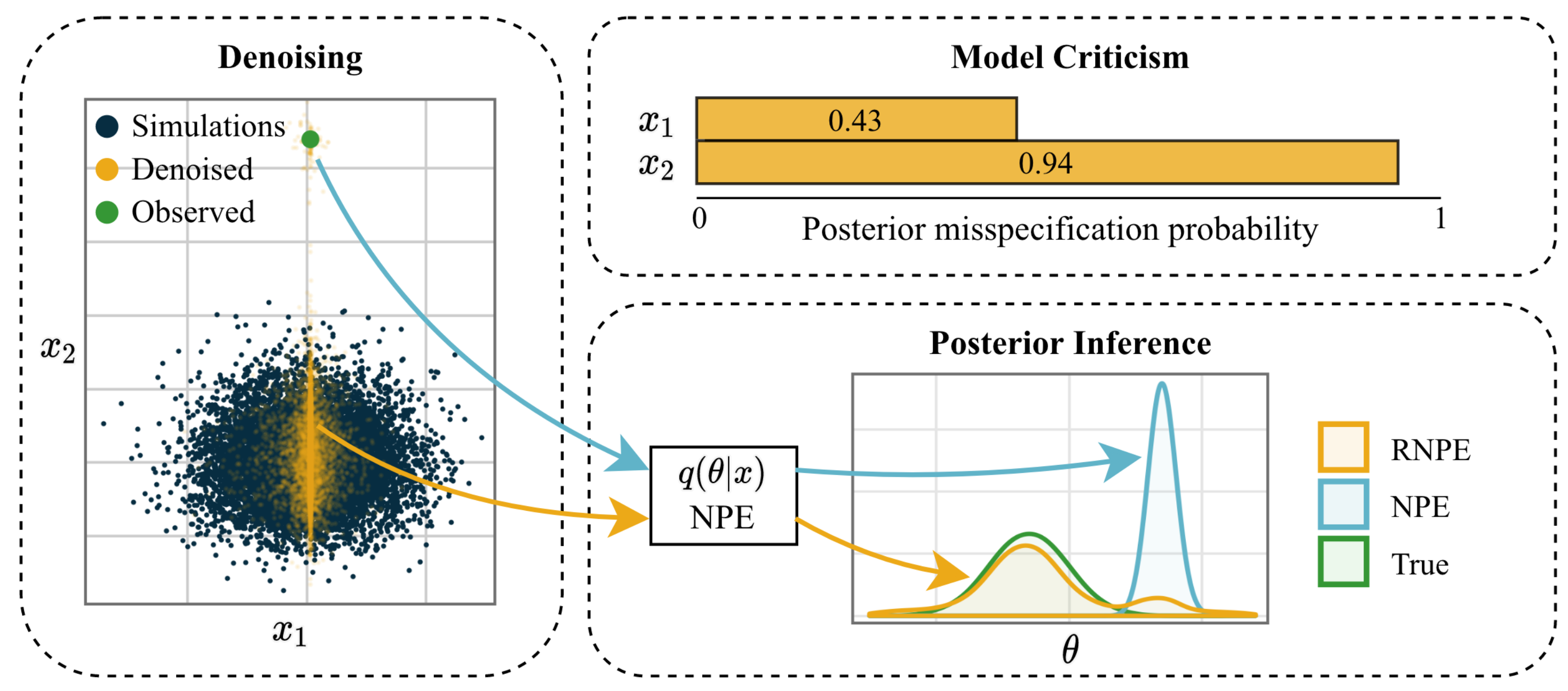
Figure 1 (adapted from [War22R]): Visualization of the robust neural posterior estimation (RNPE) framework.
Ward et al. (2022) [War22R] propose Robust Neural Posterior Estimation (RNPE), an extension of Neural Posterior Estimation (NPE), to address misspecification by explicitly modeling discrepancies between observed and simulated data. RNPE introduces an error model, $p(\mathbf{y} | \mathbf{x})$, where $\mathbf{y}$ represents observed data and $\mathbf{x}$ simulated data. This error model captures mismatches, enabling the “denoising” of observed data into latent variables $\mathbf{x}$ that are consistent with the simulator (Figure 1).
The method trains a standard NPE on simulated data while enabling its application to potentially misspecified observed data through a denoising step. This is achieved by combining a marginal density model $q(\mathbf{x})$ trained on simulated data with the explicitly assumed error model $p(\mathbf{y} | \mathbf{x})$. The error model is parametrized and trained alongside the NPE density estimator. Using Monte Carlo sampling, the denoised latent variables $\mathbf{x}_m \sim p(\mathbf{x} | \mathbf{y})$ are obtained and used to approximate the posterior $p(\theta | \mathbf{x}_m)$.
The results presented in [War22R] demonstrate that RNPE enables misspecification-robust NPE across three benchmarking tasks and an intractable example application. By explicitly modeling the error for each data dimension, the approach also facilitates model criticism, allowing practitioners to identify features in the data that are more likely to be misspecified. However, the method relies on selecting an appropriate error model, such as the “spike-and-slab” model, which may not generalize to all misspecification scenarios. Furthermore, the approach is computationally intensive, requiring additional inference steps, and is most effective in low-dimensional data spaces.
Detecting Misspecification with Learned Summary Statistics
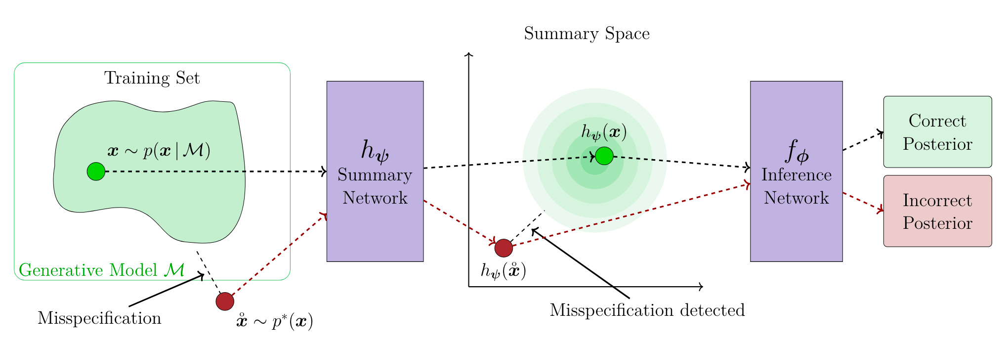
Figure 2 (adapted from [Sch24D]): Simulated data is used to train a neural network to map into a latent space designed to detect misspecification. At inference time, the observed data is embedded mapped into the latent space to detect misspecification.
Schmitt et al. (2024) [Sch24D] focus on detecting misspecification using learned summary statistics. Their method employs a summary network, $h_\psi(\mathbf{x})$, to encode both observed and simulated data into a structured summary space, typically following a multivariate Gaussian distribution (Figure 2). Discrepancies between distributions in this space are quantified using metrics like Maximum Mean Discrepancy (MMD), with significant divergences indicating misspecification.
The training procedure for this approach remains the same as in standard neural SBI methods except for an additional MMD term in the NPE loss function:
$$ \mathcal{L}_{\phi, \psi} = \mathcal{L}_{\text{inference}}(\phi) + \lambda \cdot \text{MMD}^2[p(h_{\psi}(\mathbf{x})), \mathcal{N}(\mathbf{0}, \mathbb{I})]. $$
Intuitively, the additional MMD loss term encourages the embedding network to obtain a Gaussian structure in the latent summary space, while not directly affecting the quality of the posterior estimation ensured by the standard NPE loss [Sch24D]. At inference time, the learned embedding network can then used to detect misspecification for unseen, e.g., observed, data points.
This approach is adaptable to diverse data types and does not require explicit knowledge of the true data-generating process. Additionally, it is amortized, i.e., it can be applied to new observed data without re-training because the training does not depend on $x_o$. However, its performance depends on the design of the summary network and the choice of divergence metric. While effective for detecting misspecification, it does not directly correct for it, instead providing insights for iterative simulator refinement.
Learning Misspecification-Robust Summary Statistics
Huang & Bharti et al. (2023) [Hua23L] propose a method for learning summary statistics that are both informative about parameters and robust to misspecification. Their approach is similar to the detection approach above in that it extends the standard NPE loss with an MMD term. However, this term directly takes into account the embedded observed data and balances robustness to misspecification with informativeness [Hua23L]:
$$ \mathcal{L} = \mathcal{L}_{\text{inference}} + \lambda \cdot \text{MMD}^2[h_{\psi}(\mathbf{x}_s), h_{\psi}(\mathbf{x}_o)]. $$
Here, $h_\psi$ represents the summary network, $\mathbf{x}_{s}$ and $\mathbf{x}_{o}$ are simulated and observed data, respectively, and $\lambda$ controls the trade-off between inference accuracy and robustness. Unlike the detection method above, this approach directly adjusts the summary network during training to mitigate the impact of misspecification on posterior estimation.
Benchmarking results presented in Huang & Bharti et al. (2023) demonstrate improved performance compared to the RNPE approach, with the additional advantage of applicability to high-dimensional data. However, the method has several limitations. The modified loss function introduces additional complexity, and its success depends on selecting appropriate divergence metrics and regularization parameters, which often require domain-specific tuning. Additionally, the learned embedding is tailored to a specific $x_o$ so that the method its ability to amortize over different observations. Furthermore, because robustness is implicitly learned during training and operates in the latent space, there is limited direct control over how and where misspecification is mitigated.
Addressing Misspecification with Optimal Transport
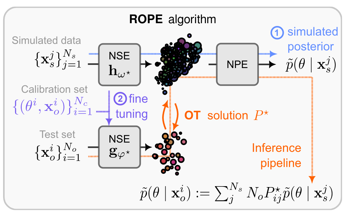
Figure 3 (adapted from [Weh24A]): Visualization of ROPE; the top line shows the standard NPE approach of learning an embedding network and a posterior estimator. Additionally, a calibration set is used to fine-tune the embedding network for embedding observed real-world data, and to learn an optimal transport mapping. At inference time, the OT mapping is used to obtain a misspecification-robust posterior estimate as a weighted sum of NPE posteriors.
Wehenkel & Gamella et al. (2024) [Weh24A] propose a method called ROPE that combines Neural Posterior Estimation (NPE) with optimal transport (OT) to address model misspecification. Their approach is designed for specific scenarios where a calibration set of real-world observations and their corresponding ground-truth parameter values is available. For instance, this may occur in expensive real-world experiments where ground-truth parameters can be measured, while a cheaper but misspecified simulator models only parts of the underlying processes. The calibration set is used to learn an optimal transport map $T$ that aligns simulated and observed data distributions.
The method begins by applying standard NPE to the simulated (misspecified) data to train an embedding network $h_\psi(\mathbf{x}_s)$ and a posterior estimator $q(\theta | \mathbf{x}_s)$. Next, the embedding network is fine-tuned on the labeled calibration set, resulting in a modified embedding network $h_\phi(\mathbf{x}_o)$ tailored to the observed data. This fine-tuned network ensures that embeddings for observed data align better with those for simulated data (Figure 3).
At inference time, a transport map $T$ is learned using OT, aligning the distributions of embedded simulated data $h_\psi(\mathbf{x}_s)$ and observed data $h_\phi(\mathbf{x}_o)$. The resulting transport matrix $P^\star$ is then used to compute a mixture model for the desired real-world data posterior:
$$ \tilde{p}(\theta | \mathbf{x}_o) = \sum_{j=1}^{N_s} \alpha_{ij} q(\theta | \mathbf{x}_s^j), $$
where $\alpha_{ij} = N_o P^\star_{ij}$, $N_o$ is the size of the calibration set, and $\mathbf{x}_s^j$ are $N_s$ simulated samples generated by running the simulator on prior parameters $\theta_j \sim p(\theta)$. The weights $\alpha_{ij}$ from the OT solution combine the posteriors $p(\theta | \mathbf{x}_s^j)$, providing a robust posterior estimate for the observed data $\mathbf{x}_o$.
An interesting property of this approach is that as $N_s$, the number of simulated samples, grows, the mixture posterior $\tilde{p}(\theta | \mathbf{x}_o)$ approaches the prior $p(\theta)$. This underconfidence property provides a mechanism to ensure that posterior estimates remain conservative and avoid overconfidence in the presence of severe misspecification. However, this effect introduces a trade-off: while increasing $N_s$ improves robustness to misspecification, it also reduces the informativeness of the posterior, potentially leading to overly broad parameter estimates. Selecting $N_s$ appropriately is therefore crucial, as it balances reliability and uncertainty quantification against the ability to extract meaningful parameter constraints (see [Weh24A] for heuristics).
While conceptually elegant and flexible, this method relies on access to calibration data—observed data with known ground-truth parameters—which may not be available in fields like cosmology or neuroscience. This reliance on calibration data limits its applicability to specific use cases.
Summary of Approaches
The methods discussed above tackle different facets of model misspecification in SBI, ranging from explicit error modeling to the development of robust summary statistics and the alignment of simulated and observed data distributions. While each approach demonstrates unique strengths, their applicability varies depending on the specific misspecification scenario, computational complexity, and the availability of calibration data.
However, the diversity of definitions, notations, and evaluation settings across these works highlights the need for a unified framework to define and compare methods. Similarly, the varying hyperparameter choices, methodological complexity, and absence of standardized benchmarks make it challenging for practitioners to navigate and apply these approaches effectively. These gaps motivate the need for better methods, common definitions, accessible benchmarks, and practical user guides, as we outline below.
Open Challenges
The recent works outlined above have made significant progress in addressing model misspecification in simulation-based inference (SBI), introducing methods for detecting and mitigating its effects. However, the problem of model misspecification in SBI is far from being fully resolved. While these methods offer valuable insights and tools, we highlight key challenges that need to be addressed to further advance the field:
Better Methods for Detecting and Addressing Model Misspecification: While recent methods have improved our ability to diagnose and mitigate model misspecification, significant limitations remain. Many current techniques focus on specific aspects of misspecification, such as identifying discrepancies in summary statistics or aligning data distributions via optimal transport. However, these approaches often require additional modeling assumptions, computational overhead, or prior knowledge about the nature of the misspecification. A key challenge is to develop more flexible and scalable methods that can:
- Detect misspecification in a principled and data-driven manner, without relying on predefined summary statistics or manual tuning.
- Provide interpretable diagnostics that help practitioners understand the sources and consequences of misspecification in their models.
- Offer robust mitigation strategies that work across different types of misspecification, without requiring large amounts of additional data or computationally expensive corrections.
A Common and Precise Definition of Model Misspecification in SBI: As highlighted in this post, model misspecification in SBI can arise from different sources, including mismatches between the simulator and the true data-generating process, prior misspecification, and errors introduced by the inference procedure itself. A common and formally precise definition of these different cases is essential for unifying the field. Such a framework would provide clarity for researchers and practitioners, enabling a more systematic comparison of methods and their applicability to specific types of model misspecification.
Common Benchmarking Tasks for Evaluating Methods: Another obstacle to progress in addressing model misspecification is the lack of an established set of benchmarking tasks tailored to the different cases of model misspecification. While current evaluations often focus on specific scenarios or datasets, limiting the generalizability of conclusions, there are promising developments. For instance, Wehenkel & Gamella et al. [Weh24A] re-used tasks proposed by Ward et al. [War22R] and introduced several new tasks designed to probe different aspects of model misspecification. These efforts provide a valuable starting point, but they need to be integrated into a common benchmarking framework and made accessible through an open-source software platform. Such a framework would enable researchers to rigorously test new methods under a variety of realistic model misspecification conditions, facilitating fair comparisons and encouraging the development of approaches robust across diverse settings.
Practical Guidelines for Detecting and Addressing Model Misspecification: For SBI to be widely adopted in practice, there is a need for clear guidelines or a practitioner’s guide on how to detect and address model misspecification, e.g., similar to a Bayesian workflow as introduced in [Gel20B]. Such a guide should include recommendations for diagnosing model misspecification using available tools, selecting appropriate mitigation methods, and interpreting posterior results under potential misspecification. This would help bridge the gap between theoretical advancements and real-world applications, ensuring that practitioners can confidently apply SBI methods in the presence of model misspecification.
Addressing these challenges will pave the way for more robust and practical SBI methods capable of handling model misspecification effectively. A unified framework, rigorous benchmarks, and practical guidelines will not only advance research on model misspecification but also simplify its handling in applied settings. Together, these efforts will strengthen SBI as a reliable tool for scientific inference in complex and realistic scenarios.
