Contrastive Language Image Pre-training (CLIP) [Rad21L] has been the dominant learning approach for pre-training multimodal models in the vision-language domain. Given a set of image-text pairs, CLIP models are trained to maximize the cosine similarity between the embeddings of the image and the text. If the training dataset is large enough and well curated [Xu23D], the resulting models can achieve impressive performance on a wide range of tasks, from segmentation, to zero-shot image classification, to even image generation (e.g. as famously done in DALL-E.
The interpretability of machine learning models, and neural networks in particular, is often centered around “putting into words” why a model makes a certain decision. This has proved to be extremely challenging, with most acclaimed methods often creating a false sense of understanding, as we discuss in our series on explainable AI. However, models that are inherently multimodal offer a natural way to map image features to text and so provide a more interpretable output.
A recent paper [Gan24I] proposes a method to decompose the image representation of CLIP into a set of text-based concepts (see Figure 1). Specifically, it focuses on CLIP-ViT, which uses a Vision Transformer (ViT) as the image encoder [Dos20I].
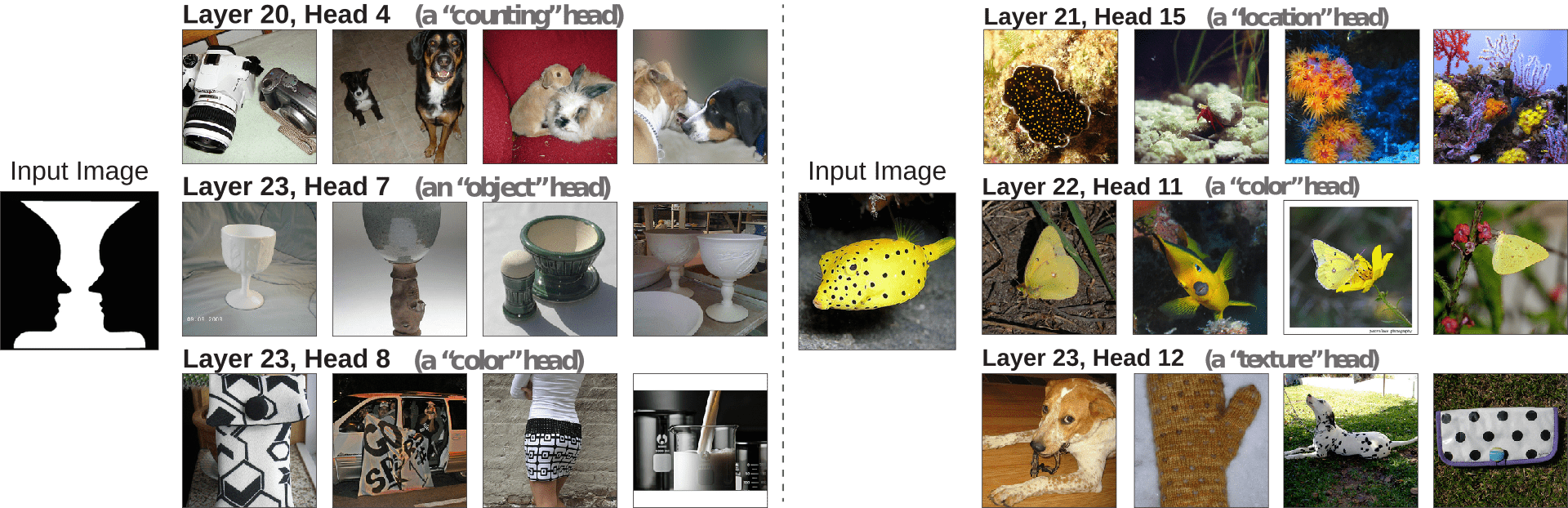
Figure 1. Some attention heads in CLIP-ViT seem to focus on extracting specific patterns. The figure shows the training images that have the highest cosine similarity with a given input image at the level of a specific attention head. For each head we can indeed find a common element, captured by a one-word textual description (Figure 5 in [Gan24I])
Given an image $I$ and text descriptions $t$, CLIP methods use two encoders, $M_{text}$ for text and $M_{image}$ for images that map to a shared latent space. During training the cosine similarity between corresponding pairs of image and text embeddings are maximized, while the similarity between non-corresponding pairs is minimized.
For image representation $M_{image}(I)$ many architectures have been studied, with ViT being one of the most successful. In short, ViT divides the image into patches, flattens them, and then processes them through a Transformer network, which is a series of multi-head self-attention layers (MSA) followed by feed-forward layers (FFN). Formally, if $Z^l$ is the output of the $l$-th layer of the Vision Transformer (with $Z^0$ the input image patches) we can write:
\begin{equation} ViT(I) = Z^0 + \sum_{l=1}^{L} \text{MSA}^l(Z^{l-1}) + \text{FFN}^l(\text{MSA}^l(Z^{l-1}) + Z^{l-1}) \tag1\end{equation}where $L$ is the total number of layers.
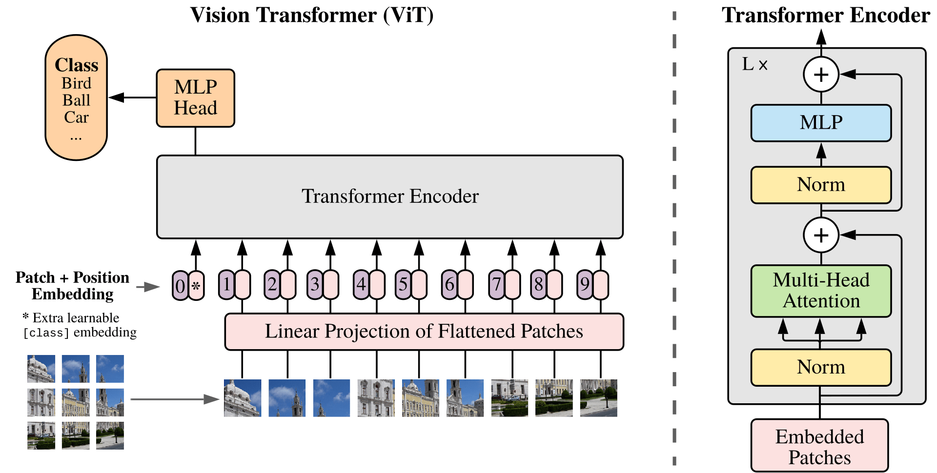
Figure 2. Representation of the Vision Transformer architecture. The input image is first split into patches, which then are projected onto a smaller space and to which positional embeddings are added. The result is fed to a standard Transformer encoder and finally to an MLP head, used for classification. (Figure 1 in [Dos20I])
Then, the Vision Transformer output is projected onto the text embedding space. So if $P \in \mathbb{R}^{d’ \times d}$ denotes the projection matrix, $M_{image}(I) = P \cdot ViT(I)$ with $d’$ chosen to be the same as the dimensionality of the text encoder output. Note that the projection matrix $P$ is learned during training. See Figure 2 for a representation of the CLIP-ViT architecture.
 Figure 3. Direct effects on model performance
of MSA layers. By progressively replacing the output of the MSA layers with
their average (cumulative, starting from early layers up to the layer indicated
on the $x$ axis), the classification accuracy only drops substantially upon
modifying the later layers. This is true for all the three ViT architectures
considered (Figure 2 in [Gan24I])
Figure 3. Direct effects on model performance
of MSA layers. By progressively replacing the output of the MSA layers with
their average (cumulative, starting from early layers up to the layer indicated
on the $x$ axis), the classification accuracy only drops substantially upon
modifying the later layers. This is true for all the three ViT architectures
considered (Figure 2 in [Gan24I])Equation 1 offers a natural way to study the direct effect of each layer of the Vision Transformer on the final image representation. One way to do this is through mean-ablation, i.e. by replacing the output of a specific component (e.g. a layer or even a single attention head) with its mean value (calculated across the training dataset) and measuring the drop in performance.
The first interesting observation of the paper is that the large majority of the direct effects in the ViT encoder come from attention layers in the later stages of the architecture (see Figure 3), while simultaneously mean-ablating the direct effects of the MLP layers only has a marginal impact on the model’s accuracy (only $1$ - $3$ % drop, see Figure 4.
The paper therefore proceeds to study only the late attention layers, and re-writes the MSA contribution in Equation 1 as: $$ \sum_{l=1}^{L} P \cdot \text{MSA}^l(Z^{l-1}) = \sum_{l=1}^{L} \sum_{h=1}^{H} \sum_{i=0}^{N} c_{l,h,i} $$ where $H$ is the number of attention heads and $N$ is the number of patches.
 Figure 4. Mean ablating all the FFN layers of the network only causes a
small drop in the zero-shot classification accuracy (Table 1 in [Gan24I])
Figure 4. Mean ablating all the FFN layers of the network only causes a
small drop in the zero-shot classification accuracy (Table 1 in [Gan24I])The contribution of the attention blocks can therefore be expressed as a sum of the $c_{l,h,i}$ terms, each of which represents a single attention head $h$ in layer $l$. Importantly, each of the $c_{l,h,i}$ is a $d’$-dimensional vector and lives in the same space as the text embeddings. Calculating the cosine similarity between $c_{l,h,i}$ and the text embedding $M_{text}(t)$ provides a natural way to interpret the effect of each component of the ViT.
At first, the paper focuses on the aggregated effects of each attention head, i.e. $c_{head}^{l,h} = \sum_{i=0}^N c_{i,l,h}$. To do so, one can take randomly selected set of input images and a large set of text descriptions $ M_{text}(t_j) $ for $j = 1, …, J $ and project $c_{head}^{l,h}$ onto the direction of each text embedding. Depending on the size of the projection, one can then identify the text descriptions that are most descriptive of the attention head. For the exact details of the implementation, refer to “Algorithm 1: TextSpan” in [Gan24I].
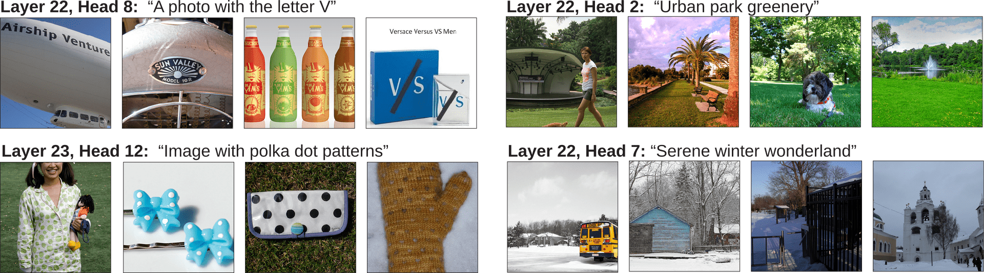
Figure 5. Examples of text representations for the reported attention heads. For each, the four images with the highest similarity between $c_{head}^{l,h}$ and the text are also reported (Figure 4 in [Gan24I])
Figures 1 and 5 show some of the results of this decomposition. Figure 6 also offers a more fine-grained analysis of the attention heads, presenting heatmaps of the image patches with the highest cosine similarity to the text embeddings.
The paper concludes with some limitations of this approach. For a start, only direct influences are studied, but the predictions of each layer do not happen in isolation and changes in the early layers can impact the values at later stages. Additional insight could come from studying higher order interactions, at the expense of simplicity and potentially interpretability.
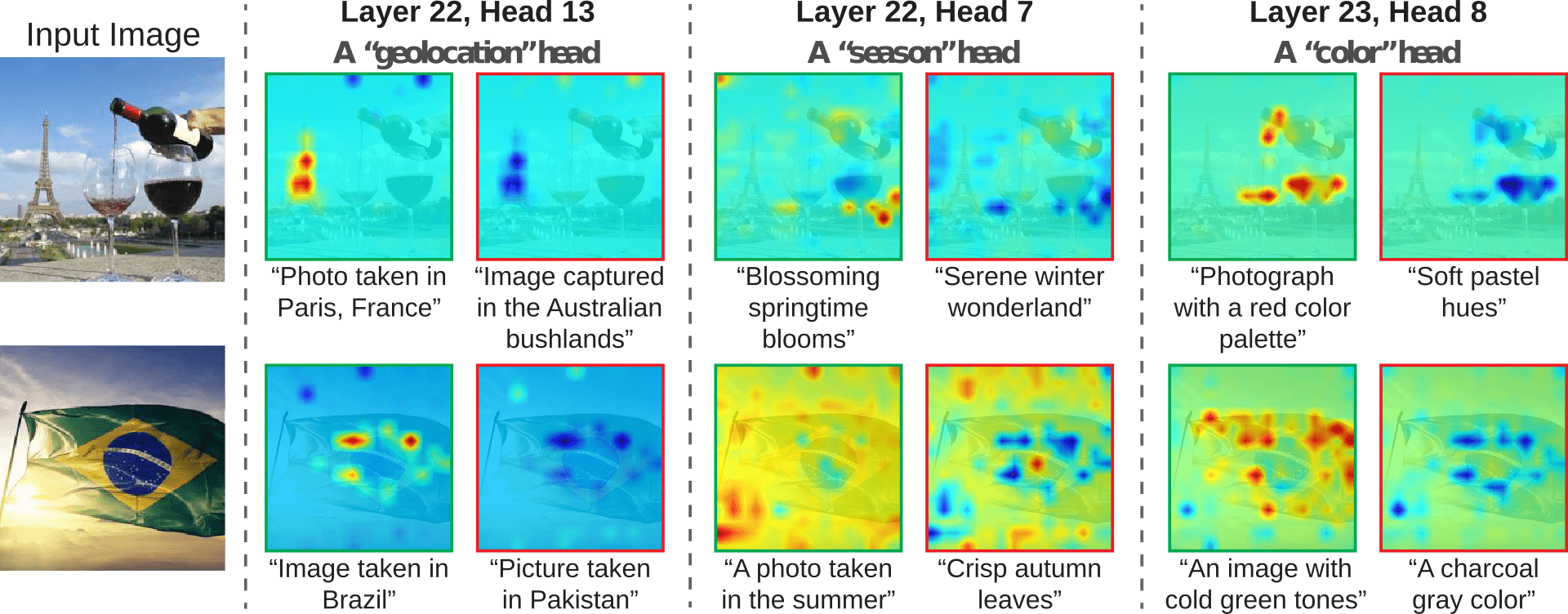
Figure 6. For the reported three heads, this image shows the descriptions with the highest (green border) and lowest (red border) similarity between $c_{head}^{l,h}$ and the provided text. Taking the top left case as an example: within this head, which specialises in geolocation, the image patches that determine that the photo was taken in Paris are also the same that negatively affect the probability that it was taken in the Australian bushlands (Figure 6 in [Gan24I])
More importantly, however, not all heads have clear roles. This can be alleviated by adding more candidate text descriptions, but there is also the chance that some parts of the model lack a coherent interpretation when taken in isolation.
CLIP models have had a remarkable impact on the field of multimodal learning, and studies like this help make them more understandable on a component by component level. The hope is that this will lead to more robust and interpretable models in the future, inverting a trend that has seen explainable AI techniques remain of limited use outside academia.
