Training data points are not created equal. No matter how clean the dataset or how simple the classification task, in real world cases some samples will always tend to be more complex than others, and therefore more complicated to learn.
Considerable effort has been devoted to understanding how ML models generalize so well to unseen samples. In doing so, the famous paper [Zha16U] observed that big neural networks tend to memorize large portions of the training dataset, including those samples that are dominated by noise (e.g. lower resolution images for computer vision). The general belief is that such behavior is bad because it deviates from what we consider optimal information extraction and compression, all things which neural networks are supposed to excel at.
Nevertheless, if in these experiments we remove all these “harder” training samples, the overall performance of the model decreases substantially. So why is memorizing training samples so ubiquitous and effective? The recent paper [Fel20W] investigates the idea that, whenever dealing with datasets coming from the real world, such as images or language, their distribution is naturally long-tailed, i.e. they tend to have a big fraction of samples which are somewhat atypical.
In order to investigate this quantitatively, the paper defines a few key metrics, the memorization and influence score, and with them analyzes the results coming from ResNet trained on ImageNet, CIFAR-100 and MNIST.
Given a model $\mathcal{A}$ (e.g. a neural network, randomly initialized), trained with a certain algorithm (e.g. gradient descent) and a dateset $S=((x_1, y_1), \dots, (x_n, y_n))$, the memorization score of $\mathcal{A}$ on a sample $(x_i, y_i) \in S$ is defined as:
$$ \text{mem} (\mathcal{A}, S, i) = P_{h \leftarrow \mathcal{A}(S)} [h(x_i)=y_i]- P_{h \leftarrow \mathcal{A}(S ^ {\backslash i})} [h(x_i)=y_i] $$
where $S^{\backslash i}$ is the dataset without $(x_i, y_i)$, $P$ is the probability over the randomness of the training process of $\mathcal{A},$ and $h(\cdot)$ represents the model prediction. In words, memorization quantifies the difference in the probability that model $h$ predicts the right label for point $i$ when $i$ is in the training set compared to when it is not.
Another very important quantity is the influence that a training sample $i = (x_i, y_i)$ has on the prediction of the model on test sample $z=(x, y)$. This is defined as follows:1 1 Albeit closely related, the influence score should not be confused with the influence function. For more details refer to the documentation of pyDVL: the python Data Valuation Library.
$$ \text{infl} (\mathcal{A}, S, i, z) = P_{h \leftarrow \mathcal{A}(S)} [h(x)=y]- P_{h \leftarrow \mathcal{A}(S ^ {\backslash i})} [h(x)=y] $$
From this, one can see $\text{mem} (\mathcal{A}, S, i) = \text{infl} (\mathcal{A}, S, i, i)$. The main issue with these definitions is that the model $h$ (a large CNN in this case) needs to be trained several (hundreds of) times, which is computationally very intensive. To speed this up, the authors only train the models on small subsets of the full dataset $S$.
The first result is that, as anticipated, if we remove samples with high memorization from the training set the overall accuracy decreases more rapidly than with random removals.
Figure 1. Accuracy on test set removing images with high memorization (Figure 2 in [Fel20W])
Figure 1 shows the accuracy (vertical axis) on the test set when we remove all images with memorization above a certain threshold (as reported on the horizontal axis) compared to the case where we randomly remove the same amount of data. Trainset fraction is instead the fraction of the original dataset left after such removal.
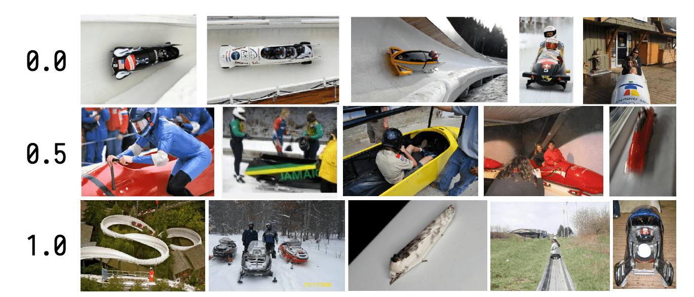
Figure 2 shows a few examples of images sorted by their memorization value.

Figure 2. Examples of images sorted by memorization (part of Figure 1 in [Fel20W])
From top line to bottom, images increase in memorization score, while at the same time becoming more atypical. Figure 3 instead shows the test images which are more highly influenced by memorized samples

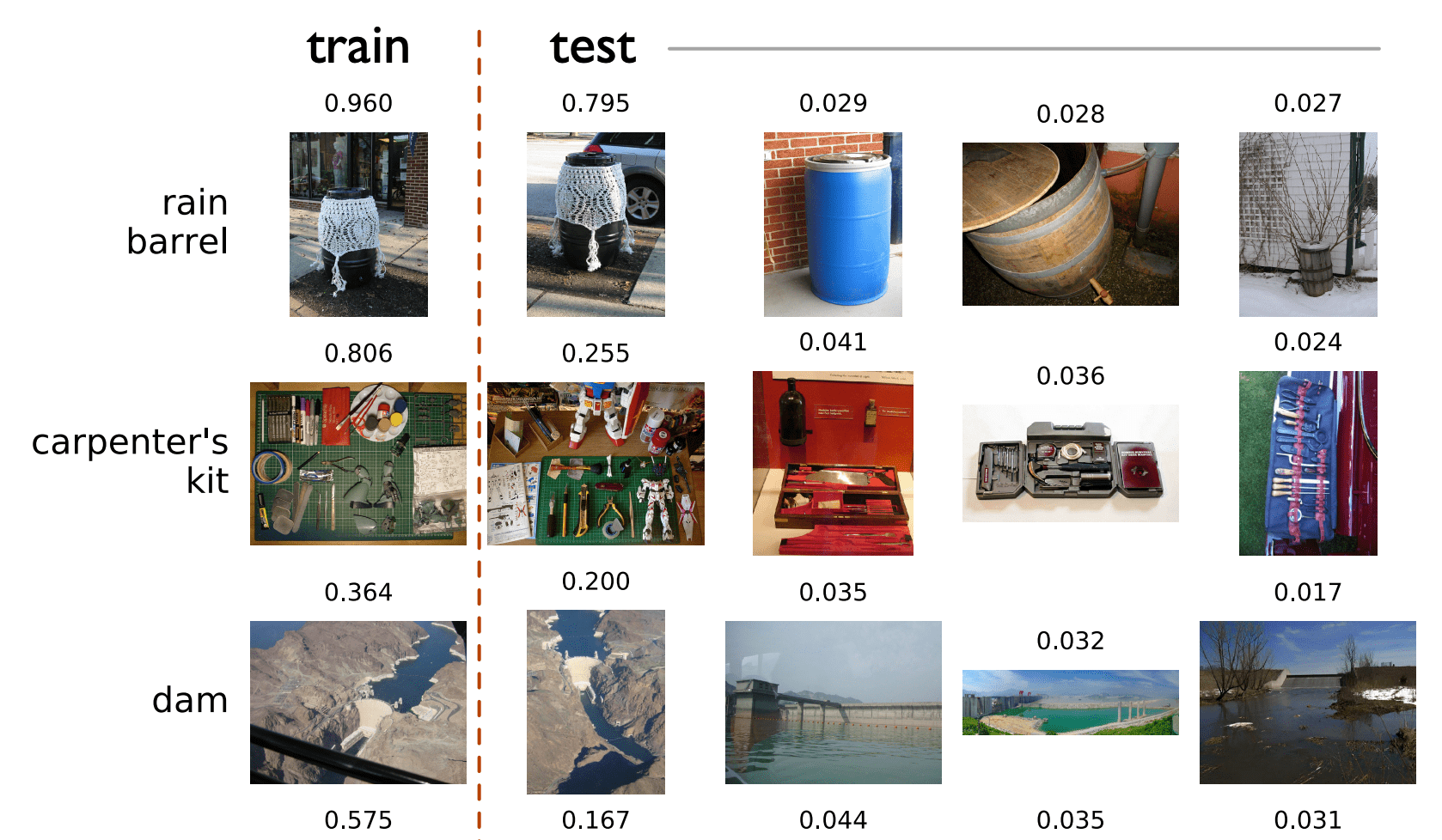
Figure 3. Highly memorized images and their influence on test images (part of Figure 6 in [Fel20W])
On the left side of the dashed line there is the training image, with relative memorization score, while on the right there are the test images, sorted in descending order of influence. Apart for the obvious cases of having the same object in training and test sets, many other images see improvements in the probability of correct prediction by 3-4 %, which then compounds to an overall big increase in total score.
To conclude, the question of what constitutes “good” data for deep learning needs to pass through a better understanding of how each sample impacts model training. The main drawback of the method here presented is the massive computational complexity that stems from repeatedly training the model. This has so far hindered a more widespread adoption of this technique, but important insight can come from it, and a faster method, albeit approximate, would be a welcome addition to the ML practitioner’s toolbox.