In recent pills, we have been closely following the development of data valuation methods. Most new ideas revolve around:

• Approximating the value (e.g. with proxy models like [Jia21S] or learned values).
• Improving the approximations (changing convergence criteria like in the seminal [Gho19D], or changing sampling strategies like in [Okh21M, Mit22S]).
• Decreasing variance (by generalizing to semi-values and putting weight on certain subset sizes with Beta shapley or improving rank stability overall in a worst-case fashion like Data Banzhaf).

The one thing that doesn’t change is the utility function of the game, which in every case is the model performance on an evaluation set, e.g. accuracy in the case of classifiers, which is the context of today’s paper:

Figure 1. Contour plot of the new utility $u = u_{y_i}.$ [Sch22C], presented at NeurIPS 2022, is very different to previous work in that it changes the utility to account for the beneficial or deleterious influence that a sample has over others of its same class. This is done by decomposing it into a product of two functions: one gives priority to in-class accuracy, while the other adds a slight discount which increases as the out-of-class accuracy increases.

To fix ideas, consider a binary classification problem, a sample $x_i$ with label $y_i$ and some subset $S$ of the training data $T.$ The test data $D$ can be split into $D_{y_i},$ the samples with the same label as $x_i,$ and $D_{-y_i},$ the samples with the other label. Analogously, one has $T = T_{y_i} \cup T_{-y_i}.$ Trained over $S$ the model has in-class accuracy:

$$a_S(D_{y_i}) := \frac{\text{# correct predictions over }D_{y_i}}{|D|},$$

and out-of-class accuracy:

$$a_S(D_{-y_i}) := \frac{\text{# correct predictions over }D_{-y_i}}{|D|}.$$

Consider now some arbitrary set $S_{-y_i} \subset T_{-y_i},$ the set of all training samples with class other than $y_i.$1 1 The set $S_{-y_i}$ is an out-of-class environment for any $S_{y_i} \subset T_{y_i}.$ Later we will average over all such environments For any set $S_{y_i} \subset T_{y_i},$ the conditional utility conditioned on $S_{-y_i}$ is defined as:

$$u(S_{y_i} | S_{-y_i}) := a_{S}(D_{y_i}) \exp \{a_{S}(D_{-y_i})\},$$

where $S := S_{y_i} \cup S_{-y_i}.$2 2 There is a problem with the original notation in the paper: In p. 4 it is stated that $S_{-y_i}$ is the complement in $S$ of $S_{y_i},$ which is wrong. Instead $S_{-y_i}$ is an arbitrary subset of the set of all training samples with label other than $y_i$ Because $a_S(D_{y_i})+a_S(D_{-y_i}) \le 1,$ this results in the second term always “pulling” the first: for fixed $a_S(D_{y_i}),$ an increase in $a_S(D_{-y_i})$ results in lower $u(S),$ see Figure 1.

With this, the conditional CS-Shapley value is:

$$\phi _{|S_{- y_{i}}}(i) := \sum_{S_{y_{i}} \subset T_{y_{i}} \backslash \lbrace i \rbrace} \binom{n - 1}{| S_{y_{i}} |}^{-1} [u_{y_{i}} (S_{y_{i}} \cup \lbrace i \rbrace |S_{- y_{i}}) - u_{y_{i}} (S_{y_{i}} |S_{- y_{i}})],$$

and the full CS-Shapley value is an average over all possible out-of-class environments:

$$v (i) := \frac{1}{2^{| T_{- y_{i}} |}} \sum_{S_{- y_{i}} \subset T_{- y_{i}}} \phi _{|S_{- y_{i}}}(i).$$

In practice, this sum is approximated with a few hundred $S_{-y_i}$ and sampling is not done from the powerset but following the usual approach cycling through random permutations and stopping whenever adding points does not increase the utility (introduced in [Gho19D]).

Section 4 of the paper goes on to show that among the class of utilities factoring as a product of two functions, one depending on the in-class accuracy, and the other depending on the out-of-class accuracy, the choice $a_{S}(D_{y_i}) \exp \{a_{S}(D_{-y_i})\}$ is the only one to fulfill certain reasonable desiderata. However, the actual value of such a proof may be questionable, since the desired properties are exactly tailored to be fulfilled by the chosen utility.

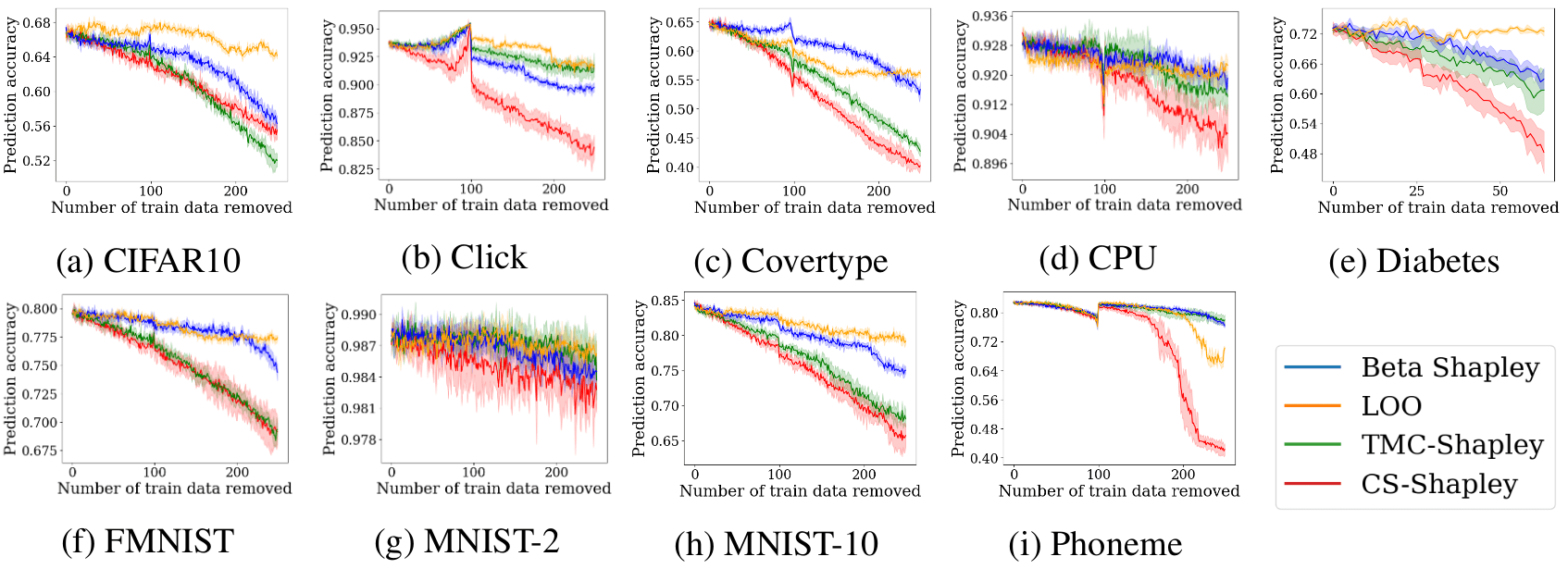
At any rate, CS-Shapley does perform greatly over multiple datasets when pitched against Truncated Monte Carlo [Gho19D], Beta Shapley and Leave-One-Out using logistic regression and SVMs. To show this, the authors propose a metric which summarises the effect of high-value data removal as a scalar by weighting the drop in accuracy after dropping a sample with the inverse of its rank. The results are summarised in Figure 2.

Finally, the authors evaluate the possibility of using Shapley values computed for a classifier as values for another one. They do this by performing the data removal test for the second classifier, using the ranking provided by the values computed for the first one. The results can be seen in Figure 3.