In Computer Vision an adversarial sample is defined as a perturbed image $\mathbf{x}’ \in \mathbb{R}^{n \times n} \mathcal{ }$ constructed from the original image $\mathbf{x} \in \mathbb{R}^{n \times n} \mathcal{ },$ such that the perturbed image is classified differently from the original image by a model $F : \mathbb{R}^{n \times n} \rightarrow \mathbb{N} ,$ but it is still classified correctly by a human. The problem of crafting adversarial samples can thus be formulated as finding a perturbation $\mathbf{x} \mapsto \eta (\mathbf{x}) $ such that $F (\mathbf{x}) \neq F (\mathbf{x}+ \eta (\mathbf{x})),$ but which is imperceptible by humans, defined as being smaller than some $\epsilon > 0$ in a given norm.
The most common norm taken is $\ell _{p}$ [Goo15E, Kur17aA], i.e. $| \eta |_{p} \leqslant \epsilon.$ However, as [Sha18S] show, $\ell _{p}$ norms are not suitable for crafting and comparing adversarial attacks, as it is possible to craft samples that have a small $\ell _{p}$ distance from the source image, but are perceptually very different, and vice versa. To remedy this, subsequent works suggest other norms. [Won20W] propose the Wasserstein distance, which restricts the amount of pixel mass that can be moved to get one image from the other. Later, [Wu20S] and [Hu20I] independently proposed improvements to the original idea, to make it stronger and faster (to the best of our knowledge there is no comparison between these two methods, and we provide one below). Note however, that while we can compare adversarial attacks using $\ell _{p}$ distances with each other, or different attacks based on Wasserstein distance, it is not possible to directly compare $\ell _{p}$ attacks with non-$\ell _{p}$ ones in terms of the amount of perturbation.
Of course one can use misclassification, but since the goal of the adversarial attacks is to stay unnoticeable for humans, it would be very convenient to have a similarity metric that aligns with human judgment. Here, we discuss usage of so-called perceptual similarity metrics for comparing adversarial attacks, and show that they are not suitable because they can be fooled by adversarial samples.
1 Perceptual Similarity Metrics
As motivation for the metric we use, we quickly recall first how three classical similarity metrics are built. The first, SSIM aggregates rough pixel information globally. The second, MSSIM, does so in patches to allow for some locality. The third, FSIM, looks at engineered low-level features. After these, a natural step presents itself: to use learned features, as does LPIPS, or, going a bit further, an ensemble of them, in E-LPIPS.
1.1 (Mean) Structural Similarity Index (SSIM)
One of the most popular perceptual similarity metrics is the Structural Similarity Index (SSIM) [Wan04I]. Because the human visual system (HVS) attends to the structural information in a scene, SSIM separates the task of similarity measurement into three comparisons: luminance, contrast, and structure.
The means of pixel values $\mu _{x}$ and $\mu _{y}$ are used to assess the similarity in luminance between the two images, while the standard deviations $\sigma _{x}$ and $\sigma _{y}$ measure contrast, and the covariance $\sigma _{x y}$ represents structural differences. The comparison function is a function of these quantities, which under some simplifying assumptions becomes:
\begin{equation} \mathrm{SSIM} (\mathbf{x}, \mathbf{y}) := \frac{(2 \mu _{x} \mu _{y} + C_{1}) (2 \sigma _{xy} + C_{2})}{(\mu _{x}^2 + \mu _{y}^2 + C_{1}) (\sigma _{x}^2 + \sigma _{y}^2 + C_{2})}, \tag{1} \end{equation}
where $C_{1}, C_{2} > 0$ are small stabilizing terms.1 1 These are included to avoid a division by zero or by a very small denominator, and are usually defined in terms of the dynamic range of the images and small tunable constants. The authors observe that this kind of global similarity measurement may not work well, and they suggest applying the function locally in different regions of the image and then compute the mean. This is known as the Mean Structural Similarity Index or MSSIM.
\begin{equation} \mathrm{MSSIM} (\mathbf{X}, \mathbf{Y}) := \frac{1}{M} \sum_{j = 1}^M \mathrm{SSIM} (\mathbf{x}_{j}, \mathbf{y}_{j}) . \tag{2} \end{equation}
1.2 Features Similarity Index Matrix (FSIM)
[Zha11F] argue that SSIM has the deficiency that all pixels have the same importance, but the HVS attributes different importance to different regions of an image. The authors argue that the HVS mostly pays attention to low-level features, such as edges or other zero crossings, and suggest comparing two sets of features:
Phase Congruency (PC) PC is a measure of the alignment of phase across different scales of an image and is a feature that is considered to be invariant to changes in brightness or contrast. It is believed to be a good approximation to how the HVS detects features in an image because the latter is more sensitive to structure than to amount of light.2 2 According to the authors: Based on the physiological and psychophysical evidences, the PC theory provides a simple but biologically plausible model of how mammalian visual systems detect and identify features in an image. PC can be considered as a dimensionless measure for the significance of a local structure. [Zha11F]
The computation of phase congruency involves several steps (for details, see [Zha11F]). First a decomposition using wavelets or filter banks, then pixel-wise extraction of phase information, followed by a comparison of the phases.
Gradient magnitude (GM) Image gradient computation is a cornerstone of image processing, e.g. for edge detection (high luminance gradients). The GM of image $f (\boldsymbol{x})$ is the Euclidean norm of the gradient: $G (\boldsymbol{x}) := | \nabla f (\boldsymbol{x}) |_{2}.$3 3 To make notation more explicit, we consider images as maps from coordinates $\boldsymbol{x}$ to channels $f (\boldsymbol{x}) =\mathbf{x}.$
For color images, PC and GM features are computed from their luminance channels. Given images $f_{i}$ and corresponding features $\operatorname{GM}_{i}$ and $\operatorname{PC}_{i},$ $i = 1, 2,$ $S_{\operatorname{PC}},$ the harmonic mean of the $\operatorname{PC}$s, and $S_{\operatorname{GM}},$ the harmonic mean of the $\operatorname{GM}$s are combined into the Features Similarity Index score:
\begin{equation} S_{L} (\boldsymbol{x}) := [S_{\operatorname{PC}} (\boldsymbol{x})]^{\alpha} [S_{G} (\boldsymbol{x})]^{\beta}, \tag{3} \end{equation}
where $\alpha, \beta$ are parameters to tune the effect of PC and GM features.
1.3 Learned Perceptual Image Patch Similarity (LPIPS)
[Zha18U] choose a different strategy for computing similarity. They argue that internal activations of neural networks trained for high-level classification tasks, even across network architectures and without further calibration, correspond to human perceptual judgments.
To get the similarity metric between two images $\mathbf{x}, \mathbf{x}_{0}$ with a neural network $F,$ they extract features from $L$ layers and unit-normalize in the channel dimension. For layer $l$ those become $\hat{y}^l, \hat{y}_{0}^l.$ Then, they scale the activations channel-wise with vectors $w^l \in \mathbb{R}^{C_{l}}$ and compute the $\ell _{2}$ distance between the respective activations for each image. Finally, they compute the spatial average and sum channel-wise. The complete metric is:
\begin{equation} d_{\operatorname{LPIPS}} (\mathbf{x}, \mathbf{x}_{0}) := \sum_{l} \frac{1}{H_{l} W_{l}} \sum_{h, w} | w_{l} \odot (\hat{y}_{hw}^l - \hat{y}_{0 hw}^l) |_{2}^2 . \tag{4} \end{equation}
The weights $w_{l}$ are optimized such that the metric best agrees with human judgment derived from two-alternative forced choice (2AFC) test results.4 4 A 2AFC test is a psychophysical method used to measure an individual’s perception or to make decisions between two alternatives under forced conditions. It’s commonly used in sensory testing, where a subject is presented with two stimuli and is required to choose one according to a specific criterion. In the 2AFC task an image is presented to a human subject together with two distorted versions of the source image. The goal is to choose which of the altered images is closer to the original.
After tuning LPIPS, the authors evaluate several similarity metrics (including SSIM and FSIM) on a separate dataset and compute agreement of the algorithm with all of the judgments. To aggregate information, if $p$ fraction of the humans vote for image 1 and $1 - p$ fraction vote for image 2, the human will get a score of $p^2 + (1 - p)^2.$

Figure 1. Quantitative comparison. Authors show a quantitative comparison across metrics on the test sets. (Left) Results averaged across traditional and CNN-based distortions. (Right) Results averaged across 4 algorithms.
In Figure 1, we see that LPIPS has a higher 2AFC score than the SSIM or FSIM measures or the $\ell _{2}$ distance.
However, a problem with the LPIPS distance is that since it uses activations of Deep Neural Networks, it is prone to adversarial attacks itself. Hence, [Ket19E] introduced the E-LPIPS or Ensembled LPIPS. They transform both input images using simple random transformations and define:
\begin{equation} d_{\mathrm{E} \text{-LPIPS }} (\mathbf{x}, \mathbf{y}) := \mathbb{E} \left[ d_{\text{LPIPS }} (T (\mathbf{x}), T (\mathbf{y})) \right], \tag{5} \end{equation}
where the expectation is taken over a family of image perturbations. The authors claim that the E-LPIPS model is more robust but has the same prediction power.
2 Problem Setting
As previously discussed, our main goal is to determine whether perceptual metrics can be used to compare adversarial attacks in image classification. We focus on LPIPS for its popularity and because it more closely aligns with human ratings than other ones (Figure 1).
[Ket19E] showed that LPIPS is sensitive to adversarial samples, but used attacks specifically targetting it. If generic adversarial attacks for image classification transferred poorly to an LPIPS network, then LPIPS could be considered for perceptual evaluation of adversarial attacks.
Consider a target network $F_{T},$ and an attack $\mathbf{x} \mapsto \mathbf{x}’ := \mathbf{x}+ \eta (\mathbf{x})$ perturbing $\mathbf{x}$ by some $\eta$ s.t. $| \mathbf{x}-\mathbf{x}’ | < \varepsilon$ in some norm. Note that induced by the distribution of images $\mathbf{x} \sim \mathbf{X},$ one has a distribution of perturbations $\mathbf{\eta} \sim \eta (\mathbf{X}).$ We can define an attack transfer from classification to LPIPS as successful if the quantity
\[ \mathbb{E}_{\mathbf{x}, \mathbf{\eta}} [| d_{\operatorname{LPIPS}} (\mathbf{x}, \mathbf{x}+ \eta (\mathbf{x})) - d_{\operatorname{LPIPS}} (\mathbf{x}, \mathbf{x}+\mathbf{\eta}) |] \]
is large enough. To compute this, we take $\mathbf{x} \in D_{\operatorname{train}}$ and approximate $\mathbf{\eta}$ by independently sampling from the set $\lbrace \mathbf{\eta} (\mathbf{x}) : \mathbf{x} \in D_{\operatorname{train}} \rbrace.$ Using only the first moment is however less informative than comparing the full distributions of distances, e.g. with the Wasserstein metric.5 5 A simple approach here would be to use a non-parametric test like Kolmogorov-Smirnov. However, in our experiments, visual inspection and Wasserstein provided ample evidence.
That is, the classification attack transfers to LPIPS successfully when LPIPS believes the adversarial samples $\mathbf{x}+ \eta (\mathbf{x})$ to be generally much closer to, or farther apart from the source images $\mathbf{x},$ than from randomly, but not adversarially perturbed images $\mathbf{x}+\mathbf{\eta}$ (although visually very similar to the adversarial samples these are not specifically designed to fool the network on a particular sample).6 6 Here we are glossing over the fact that $\mathbf{x}+\mathbf{\eta},$ where $\mathbf{\eta}$ is sampled independently from $\mathbf{x}$ might not be as imperceptible a modification as $\mathbf{x}+ \eta (\mathbf{x}).$ Our hypothesis is that since LPIPS works on top of convolutional networks designed for image classification (i.e. VGG, ResNet, AlexNet), then adversarial samples crafted for those networks will fool LPIPS as well, and hence it cannot be used to compare adversarial attacks.
3 Experimental setup
To test out the hypothesis we design the experiment following the description above. We construct adversarial samples $\mathbf{x}’$ from source images $\mathbf{x} \in D_{\operatorname{train}},$ and samples $\mathbf{x}’’ := \mathbf{x}+\mathbf{\eta}$ which are visually similar to the adversarial samples but remain classified with the correct label (fake adversaries). Then, we will compare the distributions of the scores and if there is a significant difference in distributions, our hypothesis will be verified.7 7 There are then three sets of images: original, adversaries, and fake adversaries. We compare the distances between first and second, to the distances between first and third set.
We work with the Imagenette dataset [Fas22I], which is a subsample of 10 classes from the Imagenet dataset [Den09I]. For the attacks we consider a pre-trained VGG-11 architrecture [Sim15V] and craft adversarial samples with Projected Gradient Descent (PGD) [Kur17A], Wasserstein Attack using Frank Wolfe method with Dual Linear Minimization Oracle (FW + Dual LMO) [Wu20S], and Improved Image Wassertain attack (IIW) [Hu20I]. We use multiple tolerance radiuses $\epsilon \in [0, 1]$ for each method.
To create the fake adversaries we take perturbations at random from all those used for crafting the adversarial samples and add them to the source images:
\begin{equation} f_{i} := C_{[0, 1]} [\mathbf{x}_{i} + \eta _{j}], \label{eq-fake-adversarie}\tag{6} \end{equation}
where $\mathbf{x}_{i}$ is a source image, ${\eta _{j}}_{}$ is a perturbation sampled at random from those applied to generate adversarial samples, and $C (\cdot)$ is a clipping function. We construct 10 fake adversaries for each source image, by adding 10 different perturbations from adversarial samples. A batch size of 64 is used for all the attacks. We use the LPIPS [Zha18U] metric for computing the distances with three different pre-trained bakends: VGG-16, AlexNet [Kri12I] and SqueezeNet [Ian16S] (the distance network).8 8 We chose these distance networks for consistency with the official LPIPS implementation. The target network for all the experiments discussed here is only VGG-16. We use the implementations from the official PyTorch repository [Pas19P].
The source-code9 9 github.com/bezirganyan/adversarial_arena is open-sourced and a demo is available for interactively exploring the results.10 10 bezirganyan-aai-adversarial-arena-demo-main-58mbz2.streamlitapp.com
4 Results
4.1 Measuring effectiveness of attack transfers
As a baseline, we explore if samples built against the VGG-16 network transfer to LPIPS with a VGG-16 backend. Taking $\epsilon = 0.05$ (the smallest we used for the PGD attack) we obtain a misclassification rate of 0.99 on adversarial samples and 0.072 on fake adversaries (recall: perturbed but not adversarial). The LPIPS score distributions are shown in Figure 2.

Figure 2. LPIPS score distributions for PGD attack with $\epsilon = 0.05.$ Backend: VGG-16.
As expected, we see that LPIPS scores on adversarial samples tend to be higher than on fake samples, and quite unsurprisingly conclude that LPIPS metrics with a VGG-16 backend cannot be used for comparing adversarial attacks against VGG-16 networks, as the LPIPS metric itself is affected by adversarial perturbations.11 11 For adversarial samples we only take into account those which were succesful attacks, and for the fake adversaries only perturbed images which did not misclassify (successful fake attacks). Hence, when the cardinality of either of the sets is low, we will have lower number of samples, and hence, bigger bins for the histograms.
However, what if we use LPIPS with other backend networks? From the transferability property of adversarial attacks to different networks we hypothesize that these metrics will be affected as well. To test this, we run the same experiment using AlexNet [Kri12I] and SqueezeNet [Ian16S] as backends for LPIPS. Whether or not the classification of an adversary is correct is determined by these target networks.
In Figure 3 we have the LPIPS scores with an AlexNet backbone. We can see that the distributions are much closer and have a much smaller Wasserstein distance of 0.005, compared to the 0.181 with the VGG backend. In Figure 4 we observe a similar pattern.
From these plots we hypothetise that our initial assumption was incorrect, and the $\ell _{\infty}$-PGD adversarial attacks do not trasfer to LPIPS with these backends. However, in order to be able to use this metric for comparing PGD with Wasserstein methods, we must check transferability for the latter as well.

Figure 3. LPIPS score distributions for PGD attack with $\epsilon = 0.05.$ Backend: AlexNet.

Figure 4. LPIPS score distributions for PGD attack with $\epsilon = 0.05.$ Backend: AlexNet.
4.2 Can we use LPIPS to compare Wasserstein and $\ell _{p}$ attacks?
To make our experiments with Wasserstein attacks comparable, we use an $\epsilon$ that yields a VGG-16 misclassification rate similar to the one obtained with the PGD attack (98.94%).

Figure 5. LPIPS score distributions for FW+Dual LMO attack with $\epsilon = 0.0335.$ Backend: AlexNet.
In Figures 5, 6, 7, and 8 we can clearly see that Wassertein attacks on VGG-16 transfer succesfully to other networks and hence affect the LPIPS score. This indicates that the LPIPS perceptual metric cannot be used for comparing Wasserstein adversarial attacks with other adversarial attack methods.

Figure 6. LPIPS scores distributions for FW+Dual LMO attack with $\epsilon = 0.0335.$ Backend: SqueezeNet.

Figure 7. LPIPS scores distributions for IIW attack with $\epsilon = 0.32143.$ Backend: AlexNet.

Figure 8. LPIPS scores distributions for IIW attack with $\epsilon = 0.32143.$ Backend: SqueezeNet.
5 Conclusions
In this article we investigated whether adversarial attacks can be compared using LPIPS. We crafted adversarial samples against the VGG-16 network, and also crafted non-adversarial samples with similar perturbations, which are classified correctly. Comparing the LPIPS score distributions between the source images and the adversarial samples, and source images and the perturbed but not adversarial images, we observed that the distributions are significantly different from each another, which suggests that although the perturbations were similar, the adversarial perturbation changed the activation values in a way that makes LPIPS not suitable for comparing adversarial attacks, since it is also being fooled. Thefore, human surveys are still necessary for now.
We also saw that while for PGD attacks with $\ell _{\infty}$ norm the attack did not transfer well to LPIPS with other networks as backends, Wasserstein attacks achieved much higher transferability. This is a point in favour of Wasserstein attacks, since the attacker can create samples without knowing the underlying architecture of the target network, and still hope for good results.
Appendix A: Comparing FW+Dual LMO and IIW attacks
As we mentioned earlier, to the best of our knowledge there is no comparison between the FW+Dual LMO [Wu20S] and IIW [Hu20I] attacks, although they both are improvements of the original Wasserstein Attack [Won20W]. We report in passing a quick comparison of duration and misclassification rate as a function of budget $\epsilon > 0.$ We run the attacks on the same set of images from ImageNette using their default parameters.


Figure 9. Misclassification rates and Time (sec/batch) of Wasserstein attacks as a function of budget $\epsilon.$
In Figure 9 we see that FW+Dual LMO has much better misclassifcation rate, but IIW finds adversarial samples much faster for larger budgets, while the difference of durations is comparably very small for FW+Dual LMO attacks. On average the IIW attack is almost twice as fast (329 sec/batch) than FW+Dual LMO (902 sec/batch). From Figures 7, 8, 9, and 10, we can say that IIW attempts smaller changes to the activations, but also achieves lower misclassification rate, while FW+Dual LMO makes bigger changes and achieves a higher misclassification rate.

Figure 10. LPIPS scores distributions for IIW attack with $\epsilon = 0.0005.$ Backend: SqueezeNet.
Appendix B: Bi-modality in the distance distributions
An intriguing detail in Figures 7 and 8 is that the score distributions on adversarial images (blue) have two modes: one very close to 0, and another one beyond the mode of the fake adversaries (orange). To investigate this behaviour further, we check the score distributions of the IIW attack under different values of $\epsilon .$ For $\epsilon = 0.0005$ (Figure 10) we notice that there is only one mode for the adversarial distribution, but the scores are lower than the ones of the fake adversarial distribution.
Figure 11. Fitted
modes of the adversarial (blue) and perturbed (orange) distributions (using a
Gaussian Mixture Model, and a single Gaussian respectively), and
misclassification rate (green) for the IIW attack and VGG as LPIPS backend.
While at some point the misclassification rate plateaus, the mode of the
adversarial distribution keeps increasing.
This
indicates that under low values of $\epsilon,$ the IIW attack manages to
sucessfully create adversarial samples with smaller changes in the activations
than similar random perturbations. When $\epsilon$ increases, the attack is
allowed to add more aggressive perturbations up to the allowed budget. While
for some small set of images the activations remain small, for most of them
more perturbation changes the activations more, and hence, the blue
distribution shifts to the right as in
Figures 7
and 8. See
Figure 11 for a quick empirical check.
Another check to substantiate our reasoning behind the two modes is to visually compare images from each one. In Figures 12 and 13 we see samples from both parts of the bi-modal adversarial distribution. We can see that the ones which have LPIPS distance from source images closer to the smaller mode (i.e. $d_{\operatorname{lpips}} < 0.2$), are almost indistinguishable from the source images, while the ones with LPIPS distance closer to the second mode (i.e. $d_{\operatorname{lpips}} < 0.2$) have very noticeable perturbations.
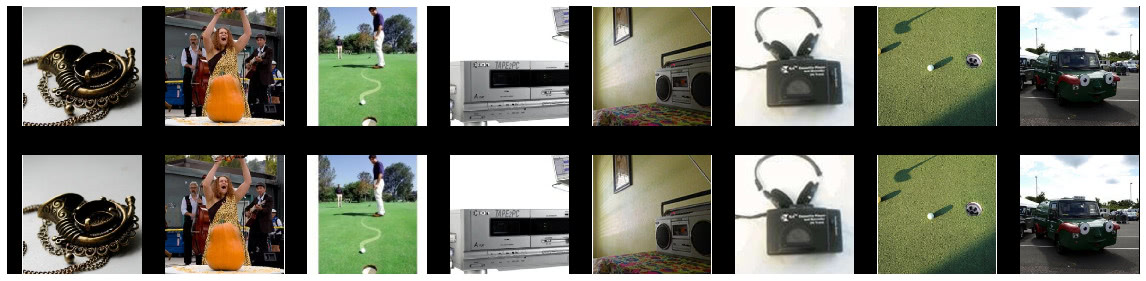
Figure 12. Adversarial samples and their source images crafted with IIW attack with $\epsilon = 0.32143,$ with low LPIPS scores between the source and the resulting adversarial sample ($d_{\operatorname{lpips}} < 0.2$).
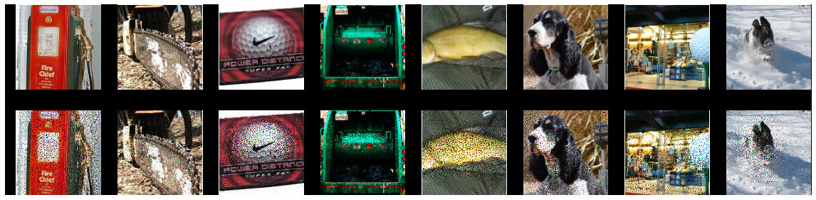
Figure 13. Adversarial samples and their source images crafted with IIW attack with $\epsilon = 0.32143,$ with high LPIPS scores between the source and the resulting adversarial sample ($d_{\operatorname{lpips}} \geqslant 0.2$).
